
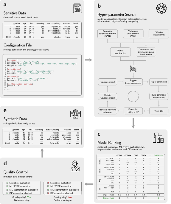
Implementation details
All DGMs evaluated in this study (CTGAN, CTAB-GAN, DP-CGANS, CopulaGAN, TVAE, TabDDPM, and TabSyn), along with the proposed correlation- and distribution-aware loss functions, were implemented using PyTorch version 1.13 (https://pytorch.org/). To ensure the reproducibility of our results, we maintained the original architectural designs and training protocols as specified in the respective publications. Additionally, to introduce variation in the comparison, we removed the conditional components from GAN-based models except for the CTAB-GAN. This was achieved by re-engineering the data sampling procedures to omit conditional vectors, thereby converting each model into its unconditional counterpart. All models were trained using the Adam optimizer42, with either default settings or parameters specified by the original authors.
Hyper-parameter tuning was conducted using the proposed IORBO framework, as detailed in ref. 31. This process was carried out in two distinct optimization stages, described in ref. 31, and aimed to ensure consistent performance across a range of datasets and model architectures.
For DP-enabled models (e.g., CTGAN, DP-CGANS and CopulaGAN), the formal privacy parameters ϵ and δ are incorporated as tunable hyper-parameters within the IORBO optimization. The optimization selects models that balance statistical fidelity, ML utility, and privacy, ensuring that the chosen models respect the computed privacy budget. Empirical post hoc DP metrics complement this formal accounting by providing practical validation of privacy protection in realistic scenarios.
All experiments were performed on a high-performance computing cluster equipped with NVIDIA A100 Tensor Core graphical processing units (GPUs) (each with 40GB of dedicated memory), Intel(R) Xeon(R) Gold 6338 CPUs, and 256GB of DDR4 RAM. Training durations varied significantly depending on the dataset and DGM complexity, ranging from a few hours up to 2 weeks.
To support efficient evaluation of downstream ML tasks, we utilized the cuML library43, which provided a GPU-accelerated Python API that closely mirrored the functionality of scikit-learn44. For consistency throughout the evaluation, we used scikit-learn to compute classification and regression metrics, scipy to derive statistical measures, and scikit-posthocs to perform statistical hypothesis testing.
For the first level (L1) and second level (L2) datasets, hyper-parameter tuning was carried out using the procedure described in “Relation to prior work”. In contrast, for the third level (L3) datasets, default hyper-parameter settings from the original implementations were used due to the substantial computational costs and GPU time requirements associated with tuning at this scale.
Relation to prior work
Several components of our methodology were built directly upon and extend our earlier work31. The foundational loss functions introduced in that work were specifically designed to align the statistical properties of synthetic data with those of real datasets. By jointly preserving pairwise correlations and marginal distributions, the proposed loss functions improved the fidelity of synthetic tabular data across diverse feature types. In this work, we retained these core formulations while integrating them more broadly into a variety of DGMs. We further demonstrated their effectiveness across new benchmarks and in-house datasets.
Correlation- and distribution-aware loss functions
Let the training dataset be defined as:
$${\bf{X}}=\{{{\boldsymbol{x}}}_{i}=({{\boldsymbol{x}}}_{i}^{(c)},{{\boldsymbol{x}}}_{i}^{(d)}):\forall i\in \{1,\ldots ,N\}\},$$
where N is the number of training samples. Each sample \({{\boldsymbol{x}}}_{i}\in {{\mathbb{R}}}^{m}\) is composed of continuous features \({{\boldsymbol{x}}}_{i}^{(c)}\) and discrete features \({{\boldsymbol{x}}}_{i}^{(d)}\).
We adopted the loss functions introduced in our previous work31, which guide DGMs to match both pairwise feature correlations and marginal distributions of the target dataset. The correlation-aware loss was defined as:
$${{\mathcal{L}}}_{{\rm{cor.}}}=\frac{2}{m(m-1)}\mathop{\sum }\limits_{j=1}^{m}\mathop{\sum }\limits_{k=j+1}^{m}{({{\boldsymbol{g}}}_{j,k}-{\widetilde{{\boldsymbol{g}}}}_{j,k})}^{2},$$
(1)
where gj,k and \({\widetilde{{\boldsymbol{g}}}}_{j,k}\) denote the sample correlation between features j and k in the real and generated datasets, respectively.
To complement this, the distribution-aware loss was given by:
$${{\mathcal{L}}}_{{\rm{dis.}}}=\frac{1}{m}\mathop{\sum }\limits_{j=1}^{m}\mathop{\sum }\limits_{h=1}^{H}\frac{1}{h}{\left(1-\frac{{\widetilde{{\mathcal{S}}}}_{j}^{(h)}+\epsilon }{{{\mathcal{S}}}_{j}^{(h)}+\epsilon }\right)}^{2},$$
(2)
where \({{\mathcal{S}}}_{j}^{(h)}\) and \({\widetilde{{\mathcal{S}}}}_{j}^{(h)}\) denote the h-th order moments of feature j computed on the real and generated data, respectively. A small constant ϵ was added for numerical stability, and H denoted the number of moments considered.
These loss functions were used alongside standard DGM objectives to guide the training process. For complete derivations, theoretical analysis, and implementation details, we referred the reader to our previous study31.
In addition to the evaluated DGMs used in ref. 31, we included TabSyn30 in this work. For the TabSyn30, the proposed loss function was integrated into the total loss of the multinomial diffusions as:
$${\widetilde{{\mathcal{L}}}}_{{\rm{TabSyn}}}={\underbrace{{{\mathbb{E}}}_{{{\boldsymbol{z}}}_{0} \sim p({{\boldsymbol{z}}}_{0})}{{\mathbb{E}}}_{t \sim p(t)}{{\mathbb{E}}}_{{\boldsymbol{\varepsilon }} \sim {\mathcal{N}}({\boldsymbol{0}},{\boldsymbol{I}})}\parallel {{\boldsymbol{\epsilon }}}_{\theta }({{\boldsymbol{z}}}_{t},t)-{\boldsymbol{\varepsilon }}{\parallel }_{2}^{2}}}_{{{\mathcal{L}}}_{{\rm{TabSyn}}}}+\alpha {{\mathcal{L}}}_{{\rm{cor.}}}+\beta {{\mathcal{L}}}_{{\rm{dis.}}},$$
(3)
where \({{\mathcal{L}}}_{{\rm{TabSyn}}}\) denotes the original TabSyn achieved via denoising score matching45.
Hyper-parameter optimization
We continued to employ the IORBO framework31 for hyper-parameter tuning, which integrated Bayesian optimization with iterative target refinement to effectively explore complex, non-convex objective landscapes. Specifically, we leveraged the tree-structured Parzen estimator approach (TPE) algorithm46 implemented in the Hyperopt (https://hyperopt.github.io/hyperopt/) library. As in our previous work, we conducted two distinct tuning processes: (1) for downstream ML tasks, we fine-tuned each model using five-fold cross-validation on task-specific evaluation metrics, and (2) for DGM, we optimized hyperparameters for each generator-dataset-loss combination. In this work, we extended the optimization objective to include additional regularization terms and downstream utility metrics, improving the flexibility and robustness of the tuning process.
Statistical tests
In our statistical analysis, we followed standard practices for hypothesis testing as outlined in ref. 31. Specifically, we interpreted p values using common thresholds for significance: p ≤ 0.01 indicated highly significant results, 0.01 < p ≤ 0.05 indicated moderate significance, and p > 0.05 suggested insufficient evidence to reject the null hypothesis. For comparing loss functions across generative models and datasets, we employed the Friedman test47—a non-parametric alternative to repeated-measures ANOVA—for ranking the methods based on two key metrics: test set predictions and statistical similarity between real and synthetic data. To identify significant differences between the ranked methods, we performed post-hoc pairwise comparisons using the Nemenyi test48. The results of these tests were summarized in ref. 31, where p values corresponded to both positive and negative differences across methods.
Evaluation
Our evaluation protocol (see Supplementary Material Fig. S4a) was built upon the comprehensive framework introduced in ref. 31, where we quantified the statistical similarity between real and synthetic datasets using distributional and correlation-based measures. Consistent with this prior work, we again applied non-parametric hypothesis tests (e.g., KS, Chi-squared) and effect size measures to assess differences in individual variable distributions and pairwise dependencies. We further evaluated ML performance on both Train-Synthetic-Test-Real (TSTR) and augmentation tasks, using a broad suite of classification and regression metrics under cross-validation.
In this work, we extended the framework in two directions to improve practical utility and robustness. First, we integrated DP risk assessments to quantify the re-identification risk of synthetic samples, offering a privacy-preserving perspective. Second, we explicitly evaluated ML performance under class imbalance, using metrics such as balanced accuracy, G-mean, and AUC to assess robustness in skewed-label scenarios. These additions, detailed in Imbalance-Aware Learning and Evaluation-3 and Supplementary Material Table S4a, supported a more realistic evaluation of synthetic data in privacy-sensitive and imbalanced-data contexts.
Benchmarking framework
Finally, the benchmarking framework used to assess model utility was adapted from ref. 31, which provided a standardized framework for evaluating DGMs across classification, regression, and statistical similarity tasks. In the present work, we expanded this framework to handle imbalanced datasets and privacy-aware applications (see Fig. S4 in the Supplementary Material), ensuring that both utility and privacy were jointly assessed. Together, these refinements represented a natural evolution of our earlier contributions, broadening their scope and strengthening their relevance to privacy-preserving data synthesis.
Dataset generation
Datasets are generated from sensitive biobank data through a three-level process that progressively transforms raw health records into analysis-ready representations (see Fig. 1). The pipeline begins with data cleaning and harmonization, followed by structured transformation and refinement for downstream use. These stages are denoted as Level 1, Level 2, and Level 3.
First level
The generation of the first level biomedical datasets involved a systematic transformation of raw data from the PREDICT, cancer registry, and consent records to create a unified, anonymized dataset suitable for subsequent analysis (see Fig. 1). The process commenced with the integration of three distinct tabular datasets into a single framework through an outer merge based on a unique patient identifier, ensuring comprehensive representation of patient information. To enhance relevance, the dataset was refined to include only individuals recruited in the PREDICT cohort, identified by a specific cohort indicator. Temporal attributes, such as birth, sampling, questionnaire, death, and vital status dates, were converted into life span metrics by calculating year differences, with age determined as the maximum available span.
Subsequent steps focused on structuring and anonymizing the data to safeguard sensitive information while preserving analytical value. Dates were grouped into 5-year intervals to reduce granularity and protect individual identities, while life span metrics underwent similar categorization to support aggregated analysis. To mitigate sparsity and ensure statistical robustness, records with infrequent occurrences of categorical variables-such as geographic locations and diagnostic codes-were excluded if their unique patient identifier counts were below a threshold of 5. Sensitive fields, including diagnostic classifications and project identifiers, were pseudonymized by encoding categorical values into numerical representations, and the patient identifier was randomized, renumbered, and reformatted to further enhance anonymity. Finally, continuous variables like body mass index were rounded for consistency, and extraneous or sensitive attributes were removed, resulting in a refined dataset stored for use in downstream modeling endeavors. Algorithm 1 details the data generation procedure for first-level datasets.
Algorithm 1
Data generation for first-level datasets
1:Input: Raw datasets, patient ID, cohort ID
2: Output: Processed dataset
3: Merge datasets using patient ID
4: Filter for PREDICT cohort
5: Calculate life spans and age
6: Bin dates and spans into 5-year groups
7: Remove rare categories
8: Anonymize sensitive data
9: Clean and round data
10: Return Processed dataset
Second level
The generation of the second-level biomedical datasets involved a detailed integration and refinement of data from questionnaire, registry, journal, and metabolomics sources to construct a comprehensive dataset tailored for cancer-related analyses (see Fig. 1). The process began by importing four distinct datasets-questionnaire responses, International Classification of Diseases (ICD) registry records, patient journals, and metabolomics profiles-into a unified framework, with initial cleaning steps such as removing redundant columns like cohort identifiers and event types from the questionnaire data. These datasets, representing 50,087 unique patient identifiers from questionnaires, 14,698 from registries, 32,996 from journals, and 3284 from metabolomics, were merged sequentially, starting with a left join of questionnaire and registry data based on a common patient identifier, followed by an inner join with metabolomics data using a sample identifier linkage.
A key aspect of the preprocessing was the classification and aggregation of cancer-related information to enhance analytical specificity. Diagnostic codes from ICD7 and ICD9 systems were labeled with specific cancer types—such as prostate, breast, colorectal, urothelial and kidney, lung, pancreatic, and hematological. We used predefined code ranges and prefixes, with a final cancer column created by prioritizing ICD9 labels where available. To capture temporal variations in patient measurements, a temporal data consolidation function restructured event-based data (e.g., “exclude diet”, “height”, “total cholesterol”) into up to five chronological sets per patient, filling earlier sets with missing values where data was sparse, particularly evident in the high missingness rates (e.g., 99.92% for “exclude diet” second set).
The final preprocessing stages focused on data reduction and quality enhancement to prepare the dataset for modeling. Columns with high missingness, such as initial measurement sets (e.g., “exclude diet” or “event date”) and metabolomics variables (e.g., EDTA plasma at 91.33%), were dropped to mitigate noise, while retaining critical attributes like birthdate and death date. Text data were standardized by stripping whitespace and converting to lowercase, and the resulting merged dataset was saved for further use. Despite significant missingness in later measurement sets (e.g., 41.85% for “event date”) and cancer-related fields (e.g., 64.50% for “diagnosis date”), the process generated cancer-specific subsets (including Prostate, Breast, Colorectal, Urothelial and Kidney, Lung, Pancreatic, and Hematological), enabling targeted investigations while addressing data sparsity through strategic filtering and aggregation. Algorithm 2 details the data generation procedure for second-level datasets.
Algorithm 2
Data generation for first-level datasets
1: Input: Raw datasets (questionnaire, cancer registry, journals, metabolomics)
2: Output: Processed dataset
3: Aggregate questionnaire events by patient
4: Label cancer types using ICD-7 and ICD-9 codes
5: Merge datasets using patient ID
6: Combine cancer labels into a single column
7: Remove sensitive and redundant columns
8: Clean and standardize data
9: Save processed dataset
10: Return Processed dataset
Third level
The generation of the third-level biomedical datasets followed the same overall procedure as the Second Level but incorporated more complete data sources. To simplify disease-specific datasets, we used the ICD-9 codes truncated to three-character resolution and translated from ICD-7 where ICD-9 entries were missing. The datasets were aggregated on a per-patient basis using the first available records, after which sensitive and redundant columns were removed. The questionnaire data were exported and merged with a multiclass cancer variable based on each patient’s first available ICD-9 code, when present.
For each ICD-9 diagnosis with sufficient data, we additionally exported questionnaire datasets merged with a binary cancer indicator (set to true if the patient had ever received the corresponding diagnosis). The most prevalent diagnoses were prostate cancer (ICD-9 code 185; 2962 patients), breast cancer (code 174; 1971 patients), and colon cancer (code 153; 1077 patients). Furthermore, we exported the aggregated questionnaire data combined with the complete metabolomics collection.
In total, 11 datasets were generated under final general data protection regulation (GDPR)-compliant approval from a special regional ethical review board. Algorithm 3 summarizes the data generation procedure for the third-level datasets.
Algorithm 3
Data generation for third-level datasets
1: Input: Raw datasets (questionnaire, cancer registry, journals, metabolomics)
2: Output: Processed dataset
3: Remove rows with missing ICD codes or malignancy status benign
4: Trim ICD codes to three letters
5: Translate ICD-7 to ICD-9 for rows with missing ICD-9 codes
6: Aggregate questionnaire data by patient using the first available records
7: Remove sensitive and redundant columns
8: Clean and standardize data
9: for each unique ICD-9 code do
10: Add a Boolean cancer column to the questionnaire data and export
11: end for
12: Add a multiclass cancer column to the questionnaire data and export
13: Merge with metabolomics data and export
14: Return Processed datasets
Preprocessing pipeline for model training
Preparing high-missingness biomedical data for generative modeling requires three linked decisions: how to impute missing values, how to stabilize heavy-tailed distributions, and how to represent missingness explicitly rather than removing it. To address these challenges, we design preprocessing strategies tailored to different dataset levels, ensuring compatibility with DGMs while preserving data quality and clinically meaningful structure.
First and second level
For Level 1 and Level 2 datasets, missing values in both continuous and discrete variables were imputed with a constant value of −1, while categorical variables were encoded using one-hot representations. This preprocessing strategy had been shown to perform adequately in natural, non-sensitive datasets where the extent of missingness was limited31.
Third level
For the third-level datasets, which contained substantially higher levels of missing data, a structured preprocessing pipeline was implemented to systematically address missingness while preserving data integrity for downstream analysis. The pipeline began with the encoding of date-related features, converting them into numerical representations of days since a fixed reference point. This ensured consistency across records and facilitated the treatment of missing or malformed entries.
Continuous and date variables with missing values were imputed using the median of the observed distribution, after which a quantile transformation was applied. Unlike standard normalization, which only rescales values linearly, quantile transformation maps the data to a uniform or Gaussian distribution, reduces the impact of outliers, and produces more stable feature distributions for training DGMs.
Binary and categorical variables were processed using one-hot encoding, ensuring that each category was represented as an independent dimension. This approach avoids implicit ordinal relationships while maintaining compatibility with downstream learning algorithms.
To further enhance model interpretability, the pipeline generated indicator variables for each continuous feature to flag instances of missingness. This allows learning algorithms to capture informative patterns associated with missing data rather than discarding them. Discrete variables are retained in their original form where appropriate to ensure structural fidelity and enable accurate inverse transformations.
In the third-level datasets, only 28 of the 126 variables were continuous, meaning that the introduction of missingness indicators resulted in a relatively small increase in dimensionality. Moreover, the inclusion of these indicators does not affect the differential privacy budget, as the privacy parameter ϵ in standard differentially private training mechanisms depends on factors such as sampling rate, training iterations, and noise multiplier rather than the number of input features. In datasets with substantially larger numbers of continuous variables, indicators can also be selectively introduced only for variables with high missingness (e.g., ≥50%), which further limits dimensional growth.
Finally, the preprocessing pipeline was designed to be bidirectional, supporting reconstruction of the original data format, including data types. In particular, the quantile transformation used in the pipeline is deterministic and strictly monotonic, constructed from the empirical cumulative distribution function of each variable. When the same fitted transformer is used for inverse transformation, the mapping remains bijective within the empirical quantile grid, ensuring that each transformed value corresponds to a unique value on the original scale. This property preserves the rank ordering and distributional structure of the data during both forward and inverse transformations. This design was essential for interpretability, validation, and reproducibility of analyses. Collectively, these steps mitigated the effects of high missingness while ensuring that the datasets remained suitable for both statistical modeling and ML applications.
Algorithm 4
Preprocessing pipeline for third-level biomedical datasets
1: Input: Raw dataset with continuous, date, binary, and categorical variables
2: Output: Preprocessed dataset with bidirectional transformations
3: Encode date features as number of days since fixed reference point
4: for each continuous and date variable do
5: Impute missing values with median of observed distribution
6: Apply quantile transformation to stabilize distributions and reduce outlier effects
7: Generate missingness indicator to flag originally missing values
8: end for
9: for each binary and categorical variable do
10: Replace missing values with dedicated placeholder
11: Apply one-hot encoding to avoid implicit ordinal relationships
12: end for
13: Retain discrete variables in original form to preserve structural fidelity
14: Ensure bidirectional transformation for full reconstruction of original data types
15: Return Preprocessed dataset ready for modeling
Illustrative example
To demonstrate the preprocessing pipeline in the Third Level, we consider a fictive dataset with five patients shown in Table 1. The dataset includes a date variable (diagnosis_date), one continuous feature (blood_pressure), and one categorical feature (smoking_status). Several values are missing, indicated by n.a.
Table 1 Raw input dataset (fictive example)
The preprocessing steps were applied as follows:
(1)
Date encoding: convert diagnosis_date into the number of days since a fixed reference (e.g., 2000-01-01).
(2)
Imputation and quantile transform (continuous and date): impute missing values using the median of observed entries, then apply a quantile transformation. Unlike standard normalization, quantile transformation reshapes skewed or heavy-tailed variables toward a uniform or Gaussian distribution, thereby reducing the impact of outliers and yielding more stable inputs for generative modeling.
(3)
Missingness indicators: add binary flags to record whether a value was originally missing prior to imputation (e.g., diagnosis_q_m, bp_q_m).
(4)
Categoricals: replace missing categories with a placeholder (“Unknown”) and apply one-hot encoding.
The resulting processed dataset is presented in Table 2. Quantile-transformed values were scaled between 0 and 1 for illustrative purposes.
Table 2 Processed dataset (fictive example)Adaptive binning of sensitive data
To reveal the exact number of individuals meeting certain criteria without revealing sensitive information, we developed an adaptive anonymization algorithm based on k-anonymity49. The goal was to limit re-identification risk by ensuring that for any combination of quasi-identifiers (attributes like zip code, age, and sex), there were at least k individuals with those same attributes, preventing attackers from pinpointing a unique person. In standard k-anonymity, a dataset typically contained sensitive attributes such as diagnosis and income that should not be linkable to a specific person. These were kept, but protected indirectly by anonymizing the quasi-identifiers, commonly by suppression (removing values) or generalization (coarse-graining, for example replacing age with age groups).
While k-anonymity safeguards against identity revelations, it does not necessarily protect against the disclosure of specific attributes. This becomes problematic when attackers possessed background knowledge that could be combined with quasi-identifiers to reduce the set of possible values for the sensitive attribute. Additionally, the absence of diversity in sensitive domains could result in the exposure of personal information through homogeneity attacks, for example if all k people in a group have the same disease. An extension called l-diversity was proposed to address this by ensuring that there were at least l well-represented values for the sensitive attribute. However, the sensitive values can be skewed or semantically similar and therefore also revealing, for example all diseases belonging to the stomach or all income values being low. A further extension called t-closeness was introduced to address this, ensuring that the distance between the distribution of a sensitive attribute for each equivalence class (any combination of quasi-identifiers) and the distribution of the attribute in the whole dataset was no more than a threshold t50.
Our solution to these vulnerabilities recognized that the root of them was the split of attributes as either identifying or non-identifying when in fact all attributes were potentially identifying, depending on their prevalence in the population and on auxiliary data that the attacker might have. By treating all attributes as both quasi-identifiers and potentially sensitive, we avoided the potential vulnerabilities that l-diversity and t-closeness tried to solve, and by using a fast greedy search with fallback to an exhaustive brute force check, we ensured that no combination of filters on any column gave less than k individuals, thus protecting against both homogeneity attacks and background knowledge attacks.
The trade-off between privacy and utility was the same as for k-anonymity, where the precision or number of values for each attribute quickly dropped with the number of attributes. To keep utility, we selected a few common attributes to get an overview: birth year, BMI, sex, and smoking status.
For each non-binary attribute, we constructed bins with different levels of precision, for example birth year binned to 5-year bins, then 10-year bins, and so on. For each level, we aimed to divide the data into bins so that each bin contained roughly the same number of observations. However, the value of equal-frequency binning for optimized precision had to be balanced with the value of simple and meaningful intervals. For example, our first-level bins on birth year were decades, with the end bins adapted to include the tails with enough data points, in our case less than 1940, 1940s, 1950s, and 1960+. Our second level of bins was less than 1950 and 1950+. For BMI, we used clinically defined bins for underweight (less than 18.5), normal (18.5 to less than 25), overweight (25 to less than 30), and obesity (30 or greater). As a next level, we merged two categories at each end into normal- and overweight+.
To adapt the bins to fulfill privacy requirements, we used k = 10 for total k-anonymity, that is, k-anonymity assuming all attributes were quasi-identifiers, and iteratively coarse-grained or removed an attribute until that was fulfilled.
Algorithm 5
Adaptive binning for privacy protection
Require: Dataset D, minimum group size k, ordered candidate binners \({\mathcal{B}}\)
Ensure: Privacy-preserving dataset Dbin
1: Dbin ← apply first binner from \({\mathcal{B}}\) to each binned column
2: while not PrivacySatisfied(Dbin, k) do
3: (c*, v*, n*) ← GreedyFilter(Dbin)
4: if coarser binning exists for column c* then
5: apply next coarser binner to column c*
6: else
7: remove column c* from Dbin
8: end if
9: end while
10: return Dbin
Imbalance-aware learning and evaluation
To improve the robustness and fairness of model evaluation in imbalanced classification settings, we introduced several modifications to the previous implementation31. First, we applied class weighting to account for the unequal distribution of classes during model training. For both support vector machine (SVM) and logistic regression classifiers, we specified the parameter class_weight = ”balanced” to ensure that each class contributed proportionally to the loss, thus mitigating bias toward majority classes.
In addition, for models that support sample-specific weights (such as XGBoost), we provided a custom weight vector sample_weights_xgb_multi when available. This allowed the model to explicitly compensate for class imbalances during optimization. If no such weight vector was present, the model defaulted to standard fitting without sample weighting.
To evaluate performance under class imbalance, we adopted metrics that were sensitive to skewed class distributions. Specifically, we reported the weighted versions of precision, recall, and F1-score-each of which considered per-class performance while adjusting for class frequency. We also computed the geometric mean score (G-mean), which captured the balance between sensitivity (recall) and specificity across all classes, making it particularly effective in the presence of imbalanced data. By integrating both training-level adjustments and tailored evaluation metrics, our framework ensured a more realistic and comprehensive assessment of synthetic data utility in real-world classification problems.
Differential privacy evaluation
To assess the privacy risks of synthetic datasets, we evaluated several DP-inspired metrics that simulate different attack scenarios. The main goal was to quantify the extent to which real data records could be inferred, re-identified, or linked from the synthetic data.
Algorithm 6
Privacy verification
1: function PrivacySatisfied(D, k)
2: ok ← GreedyPrivacyTest(D, k)
3: if ok then
4: ok ← BruteForcePrivacyTest(D, k)
5: end if
6: return ok
7: end function
8: function GreedyPrivacyTest(D, k)
9: while columns remain in D do
10: (c*, v*, n*) ← GreedyFilter(D)
11: if \({c}^{* }=\varnothing\) then
12: return true
13: end if
14: if n* < k then
15: return false
16: end if
17: D ← {r ∈ D∣r[c*] = v*}
18: end while
19: return true
20: end function
21: function BruteForcePrivacyTest(D, k)
22: if no columns remain then
23: return true
24: end if
25: for each column c in D do
26: for each value v appearing in column c do
27: \({D}^{{\prime} }\leftarrow \{r\in D| r[c]=v\}\)
28: \(n\leftarrow | {D}^{{\prime} }|\)
29: if n < k then
30: return false
31: end if
32: remove column c from \({D}^{{\prime} }\)
33: if not BruteForcePrivacyTest(\({D}^{{\prime} },k\)) then
34: return false
35: end if
36: end for
37: end for
38: return true
39: end function
40: function GreedyFilter(D)
41: \({c}^{* }\leftarrow \varnothing\)
42: n* ← ∣D∣
43: for each column c in D do
44: find value v with smallest frequency n
45: if n < n* then
46: (c*, v*, n*) ← (c, v, n)
47: end if
48: end for
49: return (c*, v*, n*)
50: end function