
Full experimental setup
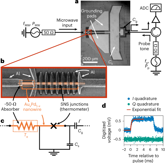
A detailed depiction of the experimental setup is shown in Extended Data Fig. 1. A NI 5782R transceiver module sent digital triggers to apply pulse modulation to a PXIe-5654 microwave source to generate the microwave pulses.
The continuous probe tone was generated by another NI PXIe-5654 microwave source. The signal was split using a directional coupler into the probe signal entering the cryostat and a reference signal. The probe tone was attenuated and filtered, and reflected off of the SNS sensor via a directional coupler. After being reflected, the signal was amplified by a Miteq high-electron-mobility-transistor amplifier at the 4 K stage of the cryostat, and then by room-temperature low-noise amplifiers. The noise temperature of the high-electron-mobility-transistor amplifier was not specified by the manufacturer at 4 K, but at 77 K it was specified to be 58.7 K with a reference temperature of 290 K. Thus, we expected the noise temperature of the high-electron-mobility transistor amplifier to be less than this at the 4 K operating temperature.
The probe signal was demodulated from radio frequency by mixing it with a local oscillator signal, which was always detuned from fp by the fixed intermediate frequency 70.3125 MHz. After demodulation, the signal was further filtered to remove sidebands from the mixing, and amplified more at the intermediate frequency.
The probe signal was digitized by the NI 5782R at a sampling rate of 250 MSa s−1 and digitally demodulated from the intermediate frequency to d.c., yielding the heterodyne in-phase (I) and quadrature-phase (Q) components. Finally, the signal was averaged and decimated over 27 adjacent samples for a digital time step of 512 ns. The reference signal was directly demodulated and digitized, and it was used as a phase reference for the digitized probe tone.
Attenuators were placed between amplifiers to avoid standing waves from reflections between the components. The 1-to-6 switches in Extended Data Fig. 1 were used to switch between the sample used in our experiment and other samples unrelated to this work.
The total input line attenuation was calibrated following the procedure introduced in ref. 52. In a separate thermal cycle of the cryostat, we replaced the SNS sensor used in the main experiment with a bolometer that could be heated both with microwave power and d.c. current. We applied a known d.c. power to the nanowire using a four-wire configuration, and by varying the radio frequency powers applied at room temperature and comparing the resulting frequency shift, we found correspondence between the room-temperature radio frequency power and the power at the chip. We found that the total input line attenuation was 119.24 ± 0.1 dB. Note that this was the total attenuation up to the input of the sample holder containing the chip used in the main experiment. Thus the reported energy resolution considered our sensor to be a black box at the end of a 50-Ω transmission line, and it included possible reflections owing to impedance mismatch at the chip input that degraded the measured energy resolution. We considered the change in line attenuation between the thermal cycles of the cryostat to be negligible.
Model for bolometric transmission
In the bolometric linear mode of operation, the steady-state reflection coefficient of the gate capacitor at a given probe frequency fp follows a Lorentzian line shape53:
$$\Gamma \propto 1-\frac{{{\rm{e}}}^{{\rm{i}}\varphi }{\gamma }_{{\rm{c}}}}{\gamma /2+2\pi {\rm{i}}\left(\,{f}_{{\rm{r}}}-{f}_{{\rm{p}}}\right)},$$
(1)
where fr is the resonance frequency of the LC tank circuit of the sensor, γc and γ are the external and total energy decay rates, respectively, and φ is a parameter corresponding to the asymmetry of the resonance owing to impedance mismatch between the chip and the coaxial cable at the probe input. The resonance frequency shifts approximately linearly with the power PMW of the microwave tone44 (or equivalently, the pulse energy EMW = PMW tMW):
$${f}_{{\rm{r}}}={f}_{{\rm{r}},0}-\alpha {P}_{{\rm{MW}}},$$
(2)
where fr,0 is the resonance frequency with no microwave pulse, and α is a coefficient with units of Hz W−1 corresponding to the conversion of PMW to heat in the absorber, and subsequently to a change in the Josephson inductance of the nanowire. In general, α depends on several factors, including the absorber geometry and material, and impedance matching of the absorber to the input coaxial line.
The difference in the complex heterodyne transmitted signal I + iQ with a given input power is thus proportional to
$$\begin{array}{l}\Gamma ({\rm{P}}={{\rm{P}}}_{\mathrm{MW}})-\Gamma ({\rm{P}}=0)\\ \propto \left(\frac{1}{{\rm{\gamma }}/2+2{\pi i}\left({{f}}_{{\rm{r}}\mathrm{,0}}-{{f}}_{{\rm{p}}}\right)}-\frac{1}{{\rm{\gamma }}/2+2{\pi i}\left({{f}}_{{\rm{r}}\mathrm{,0}}-{\mathrm{\alpha P}}_{\mathrm{MW}}-{{f}}_{{\rm{p}}}\right)}\right){{\rm{e}}}^{{i\varphi }}{{\rm{\gamma }}}_{{\rm{c}}}.\end{array}\,\,\,\,$$
(3)
The relative change in the digitized voltage ΔV is obtained by applying a rotation to cancel out φ, multiplying by the total gain of the amplification chain G, and discarding the imaginary part as
$$\begin{array}{rcl}\Delta V & = & G{\gamma }_{{\rm{c}}}\,\text{Re}\,\left[\frac{1}{\gamma /2+2\pi {\rm{i}}\left({f}_{\mathrm{r,0}}-{f}_{{\rm{p}}}\right)}-\frac{1}{\gamma /2+2\pi {\rm{i}}\left(\,{f}_{\mathrm{r,0}}-\alpha {P}_{\mathrm{MW}}-{f}_{{\rm{p}}}\right)}\right]\\ & = & G\frac{\gamma {\gamma }_{{\rm{c}}}}{2}\left(\frac{1}{{(\gamma /2)}^{2}+{\left[2\pi \left({f}_{{\rm{r}},0}-{f}_{{\rm{p}}}\right)\right]}^{2}}-\frac{1}{{(\gamma /2)}^{2}+{\left[2\pi \left(\,{f}_{{\rm{r}},0}-\alpha {P}_{\mathrm{MW}}-{f}_{{\rm{p}}}\right)\right]}^{2}}\right).\end{array}$$
(4)
With large values of PMW, this expression becomes effectively constant, and hence the energy resolution of the sensor approaches zero. However, it may still be used as a binary detector, indicating the presence or absence of a microwave signal.
Estimation of the noise PSD
The one-sided noise PSD Sn of the measured voltage is used both in calculating the NEP and in the matched-filtering procedure. We estimate the noise PSD by averaging periodograms according to Bartlett’s method54 for data with no pulse applied.
The PSD used in the matched filtering is obtained by fitting the estimated PSD to a simple heuristic model \({\widetilde{S}}_{{\rm{n}}}(f)=A/f+B\), which is a sum of 1/f and white noise. Using this model instead of the estimated PSD directly yields a better SNR, since the estimate is noisy (Extended Data Fig. 2a). The measured spectrum does not completely agree with this model, which we attribute to the analogue filtering and amplification in the output chain. Nevertheless, we find that using the model in the matched-filtering procedure improves the energy resolution by approximately 4% compared with using the raw noise PSD. Note that one may freely choose the noise model in the matched-filtering procedure without loss of scientific soundness.
Obtaining the NEP
To obtain the NEP from the experimental data in the bolometric mode, we record time-domain traces of the transmitted signal similar to the one shown in Fig. 1d for different values of fp and Pp. We offset the time axis such that t = 0 is at the arrival time of the pulse, and fit these traces to the model \(\Delta V\times (1-{{\rm{e}}}^{-t/\tau })\) for t > 0 to extract the relative-voltage signal ΔV and thermal time constant τ.
With fp close to fr,0 and αPMW ≪ γ, we have an approximately linear dependence of ΔV on PMW, and hence we define the quasistatic responsivity as δV/δPMW = ΔV/PMW, where the word quasistatic refers to the fact that this definition assumes that PMW is constant in time. To determine how the responsivity varies with temporal changes in PMW occurring at the noise frequency fn, the responsivity may be measured while modulating PMW at fn. However, we capture the frequency dependence of the responsivity by21,33,55 \(\delta V/\delta {P}_{\mathrm{MW}}{[1+{(2\pi {f}_{{\rm{n}}}\tau )}^{2}]}^{-1/2}\), which takes into account the decrease in responsivity owing to the thermal time constant τ. Note that this procedure is justified by our empirical observation in Fig. 1d that the rise of the sensor signal for PMW suddenly turned on is accurately exponential.
The NEP is thus given by
$$\,\text{NEP}\,\left(\,{f}_{{\rm{n}}}\right)=\sqrt{{S}_{{\rm{n}}}\left(\,{f}_{{\rm{n}}}\right)}{\left(\delta V/\delta {P}_{\mathrm{MW}}\right)}^{-1}\sqrt{1+{\left(2\pi {f}_{{\rm{n}}}\tau \right)}^{2}},$$
(5)
where Sn(fn) is the noise PSD of the measured relative voltage ΔV at the frequency fn. The units of the NEP are \({\rm{zW}}/\sqrt{{\rm{Hz}}}\) since it equals the square root of the noise PSD of the measured signal in units of input power to the bolometer. The NEP obtained at the operation point used for the calorimetry is shown in Extended Data Fig. 2b.
For the probe parameters considered in Fig. 2, the NEP is lowest around the range of 0.3–1 kHz, indicated by the shaded region in Extended Data Fig. 2b. In this frequency range, the effect of the 1/f noise is reduced, but the insensitivity owing to finite τ is not yet considerable. This implies that the highest sensitivity in the bolometric mode can be achieved by modulating the input power PMW at a frequency within this range, for example, by using a shutter, a multiplexer that switches between two bolometers, or by using lock-in detection. Thus we choose to average over this range for the data shown in Fig. 2c.
The NEP also allows us to estimate the energy resolution, through the relation21
$$\Delta {E}_{\mathrm{FWHM}}=2\sqrt{2\ln 2}{\left({\int }_{0}^{{f}_{\max }}\frac{4}{{\mathrm{NEP}}^{2}(\,f\,)}{\rm{d}}f\right)}^{-1/2},$$
(6)
where the factor \(2\sqrt{2\ln 2}\) arises from the used FWHM of a normally distributed signal (discussed below) and \({f}_{\max }\) is a frequency, up to which the sensor is used. In our previous work33, we have used the thermal cut-off 1/(2πτ) for the upper bound of the integral, but we find that in our case, this gives an unnecessarily pessimistic estimate. This equation is used to obtain the data shown in Fig. 2d.
Single-shot data processing using matched filtering
Here we discuss the data processing used for the data in the calorimetry experiments where no ensemble-averaging is carried out. The phase of each digitized and down-converted heterodyne trace relative to each other is normalized using a phase reference (Extended Data Fig. 1), and the baseline is removed by subtracting the median of the I and Q components of each trace for the section before the pulse. The baseline-removed traces are rotated in the I–Q plane by a global phase angle \(\widetilde{\varphi }\) such that projecting the rotated signal to the I axis yields the finest energy resolution. An example of such a digitized trace after this preprocessing step is shown in Fig. 3a.
After the preprocessing, a matched filter21,43,56 is applied to the projected in-phase signal. The matched filter is the linear time-invariant filter that maximizes the SNR, and hence it is sometimes called an optimal filter. For the matched filter, the filtered signal is given by the following convolution:
$${S}_{k}={\text{DFT}}^{-1}{\left[\frac{\text{DFT}{\left[{V}_{k}\right]}_{j}\times {\overline{\text{DFT}\left[{K}_{k}\right]}}_{j}}{{S}_{{\rm{n}},\,j}}\right]}_{k},$$
(7)
where Vk is the digitized signal at the sample index k, Kk is the template of the matched filter (discussed below), \(\overline{z}\) denotes the complex conjugate of z, \({S}_{{\rm{n}},j}={S}_{{\rm{n}}}\left({f}_{{\rm{n}},j}\right)\) is the noise PSD at the frequency bin with index j, and DFT and DFT−1 denote the discrete Fourier transform and its inverse, respectively.
The values of the signal after the matched filtering, Sk, indicate how well the raw signal and template correlate at a given convolution offset, with additional weighting from the noise PSD emphasizing frequency components that are less noisy. If the pulse arrival time is known and the template has a duration equal to the window of the digitized signal, the matched filter yields a peak at zero convolution offset. The final calorimetric signal \(\bar{S}\) is obtained by taking the mean of the filtered signal Sk over a 1.024-μs window centred at zero convolution offset, as shown in Fig. 3c.
The template of the matched filter is the expected time-domain shape of the signal, which is assumed to be directly proportional to the energy of the pulse. For the short pulses used in the calorimetry, we model the temporal dependence of the projected signal as a sum of two exponentially decaying processes as
$$K(t)=\left\{\begin{array}{ll}0 & t < 0,\\ ({a}_{1}+{a}_{2})\times t/{t}_{{\rm{MW}}} & 0\le t < {t}_{{\rm{MW}}},\\ {a}_{1}\exp \left[-(t-{t}_{{\rm{MW}}})/{\tau }_{1}\right]+{a}_{2}\exp \left[-(t-{t}_{{\rm{MW}}})/{\tau }_{2}\right] & {t}_{{\rm{MW}}}\le t,\end{array}\right.$$
(8)
where the arrival time of the pulse is t = 0 and tMW = 1 μs is the length of the pulse. The amplitude a1 and time constant τ1 correspond to a fast decay of heat from the electrons to an intermediate heat bath, and a2 and τ2 to a slow decay from the intermediate bath to the phonon bath of the chip substrate through a weak thermal link. The exact physical origin of this double-exponential behaviour is unknown, but such behaviour has been reported in earlier experiments with similar devices39,57. Here we assume a zero baseline, and that the length of the input pulse tMW is much shorter than the time constants τ1 and τ2, so that the signal rises effectively linearly during the pulse. We extract the template by ensemble-averaging 1,000 pulses with a relatively high pulse energy of 3.8 zJ and fitting the data to equation (8). From the fit, we obtain τ1 ≈ 18 μs, τ2 ≈ 150 μs and a2/a1 ≈ 1.5. The template with these parameters is shown in Fig. 3b.
With high powers, the heterodyne signal moves along a curve in the I–Q plane, as predicted by equation (3). Thus the linear relationship between the pulse energy and the projected signal ΔV breaks down, and the effectiveness of the matched filter is reduced. While we observe some deviation from the linear behaviour in our data, we find that this effect does not considerably affect the filtering procedure for the pulse energies considered here.
Conversion of filtered signal to energy units and calculation of the energy resolution
The calorimetric signal \(\bar{S}\) extracted from the matched-filtering procedure has arbitrary units, since we have not calibrated the whole amplification chain from the sample to the analogue-to-digital converter. Here we discuss the procedure used to convert the extracted signal and its standard deviation to units of energy for Fig. 4, and how that is subsequently used to obtain the energy resolution.
For each pulse energy EMW, we collect N = 1,000 traces and extract the corresponding signals \({\bar{S}}_{j}\), j = 1, …, N as discussed above. We then compute the empirical CDF for each EMW, given by
$${\text{CDF}}_{{E}_{\mathrm{MW}}}(s)=\mathop{\sum }\limits_{{\bar{S}}_{j}\le s}\frac{1}{N}.$$
(9)
The noise in the signal closely follows a normal distribution, and therefore we model the CDF for a given pulse energy E as
$${\text{CDF}}_{E}(s)=\frac{1}{2}+\frac{1}{2}\text{erf}\,\left(\frac{s-{\mu }_{\bar{S}}(E\,)}{\sqrt{2}{\sigma }_{\bar{S}}(E\,)}\right),$$
(10)
where erf( ⋅ ) is the error function, and \({\mu }_{\bar{S}}\) and \({\sigma}_{\bar{S}}\) are the mean and standard deviation of the corresponding normal distribution, respectively. We extract \({\mu }_{\bar{S}}\) and \({\sigma }_{\bar{S}}\) by a least-square fit of the error function in equation (10) to the empirical CDF.
Since we have calibrated the total attenuation at the input of the microwave absorber, the energy corresponding to each value of \({\mu }_{\bar{S}}\) is known, up to a constant relative error of ±0.1 dBm, discussed below. Since \(\bar{S}\) is proportional to δV/δPMW, its dependence on EMW is also of the form of equation (4) (with PMW = EMW/tMW and α adjusted). We invert equation (4) by solving for EMW to obtain
$${\mathcal{E}}(s)=\frac{{t}_{{\rm{MW}}}}{2\pi \alpha }\left(2\pi \left({f}_{{\rm{r}},0}-{f}_{{\rm{p}}}\right)+\sqrt{{\left[\frac{1}{{(\gamma /2)}^{2}+{\left[2\pi \left({f}_{{\rm{r}},0}-{f}_{{\rm{p}}}\right)\right]}^{2}}-\frac{s}{a}\right]}^{-1}-1}\right),$$
(11)
where a = Gγγc/2 is a scaling parameter of the measured signal corresponding to the unknown prefactor in equation (4). We fit this model to the extracted values of \({\mu }_{\bar{S}}\) with \({\widetilde{\Delta }}_{f}=({f}_{{\rm{r}},0}-{f}_{{\rm{p}}})/\alpha\), \(\widetilde{a}=a/\alpha\), and \(\widetilde{\gamma }=\gamma /\alpha\) as the fitting parameters. This then allows using \({\mathcal{E}}(s)\) as a calibration curve that maps a signal s to the corresponding energy reported by the calorimeter. Extended Data Fig. 3a shows \({\mu }_{\bar{S}}\) and \({\mathcal{E}}(s)\). To convert the standard deviation \({\sigma }_{\bar{S}}(E)\) at a given energy to the standard deviation σE(E) that is in units of energy, we use the following relation58 for the variance of a random variable transformed by a nonlinear function:
$${\sigma }_{E}^{2}\approx {{\mathcal{E}}}^{2}({\mu }_{\bar{S}})+{\sigma }_{\bar{S}}^{2}\left({\left[{{\mathcal{E}}}^{{\prime} }({\mu }_{\bar{S}})\right]}^{2}+{\mathcal{E}}({\mu }_{\bar{S}}){{\mathcal{E}}}^{{\prime\prime} }({\mu }_{\bar{S}})\right)-{\left[{\mathcal{E}}({\mu }_{\bar{S}})+\frac{{\sigma }_{\bar{S}}^{2}}{2}{{\mathcal{E}}}^{{\prime\prime} }({\mu }_{\bar{S}})\right]}^{2}.$$
(12)
The standard deviations \({\sigma }_{\bar{S}}\) obtained using equation (10) and the corresponding σE are shown in Extended Data Fig. 3a as horizontal and vertical bars, respectively, as well as in Extended Data Fig. 3b,c as crosses. The FWHM is that of a Gaussian function, given by \({W}_{E}={\sigma }_{E}\times 2\sqrt{2\ln 2}\). The data points in Fig. 4b are thus calculated as \({E}_{{\rm{MW}}}/{W}_{{E}_{{\rm{MW}}}}\).
To estimate σE between the values we have measured, we approximate \({\sigma }_{\bar{S}}(E)\) by the quadratic polynomial σs(E) = a0 + a1E + a2E2 that is fit to the measured \({\sigma }_{\bar{S}}\). We then transform this interpolated curve according to equation (12) (with \(s={{\mathcal{E}}}^{-1}(E)\) in place of \({\mu }_{\bar{S}}\)), resulting in the curve shown in Extended Data Fig. 3c. This yields the interpolated FWHM W(E), and subsequently the interpolated curve in Fig. 4b, which is given by E/W(E). Finally, the estimated energy resolution of 0.83 zJ is determined by numerically finding E such that E = W(E).
Note that the projection angle \(\widetilde{\varphi }\), as well as the averaging window discussed above are chosen such that the energy resolution estimated with this method is optimized. Nevertheless, we find that for the 0.95 zJ pulse, even if \(\widetilde{\varphi }\) is offset by up to 0.1 × 2π from its optimal value, the measured signal-to-FWHM ratio can be made greater than unity by adjusting the averaging window offset and length by 1–2 μs.
Uncertainty of the energy resolution
Here we discuss how we obtain the uncertainties of 0.02 zJ in the pulse energy 0.95 zJ and 0.04 zJ in the energy resolution estimate. It is important to make a distinction between the standard deviations σs and σE, which stem from noise in the signal and are obtained by fitting the empirical CDFs, and their uncertainties δσs and δσE, respectively, which are derived from the fit. We use uncertainty to exclusively refer to δσs and δσE, as well as to other sources of error such as the 0.1 dB of uncertainty in the calibration of the line attenuation.
We obtain the uncertainty in E/W(E) as follows:
$$\delta \left[\frac{E}{W(E)}\right]=\frac{E}{W(E)}\sqrt{{\left(\frac{\delta E}{E}\right)}^{2}+{\left(\frac{\delta W(E)}{W(E)}\right)}^{2}},$$
(13)
where δE is given by 0.1 dB × E ≈ 1.023 × E, and
$$\delta W(E)=2\sqrt{2\ln 2}\,\delta {\sigma }_{E}(E)=2\sqrt{2\ln 2}\,{\sigma }_{s}(E){{\mathcal{E}}}^{{\prime} }(s)\sqrt{{\left(\frac{\delta {\sigma }_{s}(E)}{{\sigma }_{s}(E)}\right)}^{2}+{\left(\frac{\delta {{\mathcal{E}}}^{{\prime} }(s)}{{{\mathcal{E}}}^{{\prime} }(s)}\right)}^{2}},$$
(14)
where
$$\delta {\sigma }_{s}(E)={\left[{\nabla }_{{\rm{P}}}{\sigma }_{s}(E)\right]}^{{\rm{T}}}{{\bf{C}}}_{{\sigma }_{s}}{\nabla }_{{\rm{P}}}{\sigma }_{s}(E),$$
(15)
and
$$\delta {{\mathcal{E}}}^{{\prime} }(s)={\left[{\nabla }_{{\rm{P}}}{{\mathcal{E}}}^{{\prime} }(s)\right]}^{{\rm{T}}}{{\bf{C}}}_{{{\mathcal{E}}}^{{\prime} }}{\nabla }_{{\rm{P}}}{{\mathcal{E}}}^{{\prime} }(s),$$
(16)
where \(s={{\mathcal{E}}}^{-1}(E)\) and ∇Pσs(E) denotes the gradient of σs(E) with respect to each of its parameters: \({\nabla }_{{\rm{P}}}{\sigma }_{s}(E)={[{\partial }_{{a}_{0}}{\sigma }_{s}(E),{\partial }_{{a}_{1}}{\sigma }_{s}(E),{\partial }_{{a}_{2}}{\sigma }_{s}(E)]}^{{\rm{T}}}\), and similarly \({\nabla }_{{\rm{P}}}{{\mathcal{E}}}^{{\prime} }(s)\) denotes the gradient of \({{\mathcal{E}}}^{{\prime} }(s)\) with respect to the parameters of the Lorentzian: \({\nabla }_{{\rm{P}}}{{\mathcal{E}}}^{{\prime} }(s)={[{\partial }_{\widetilde{a}}{{\mathcal{E}}}^{{\prime} }(s),{\partial }_{\widetilde{\gamma }}{{\mathcal{E}}}^{{\prime} }(s),{\partial }_{{\widetilde{\Delta }}_{f}}{{\mathcal{E}}}^{{\prime} }(s)]}^{{\rm{T}}}\), and \({{\bf{C}}}_{{\sigma }_{s}}\) and \({{\bf{C}}}_{{{\mathcal{E}}}^{{\prime} }}\) are the covariance matrices of the parameters, obtained from the fitting procedure described above. We have included the uncertainties in \({\sigma }_{\bar{S}}\) and \({\mu }_{\bar{S}}\) obtained from the CDF fitting as weights in the fitting of \({\mathcal{E}}\) and σs, so that the effect of these are included in the covariance matrices.
Note also that the Poissonian statistics of the coherent input photons cause fluctuations in the input photon number with a standard deviation of \(\sqrt{E/(h{f}_{{\rm{MW}}})}\), or equivalently, fluctuations in the energy with a standard deviation of \(\sqrt{Eh{f}_{{\rm{MW}}}}\). The effect of these fluctuations is already included in \({\sigma }_{\bar{S}}\), and hence also in the signal-to-FWHM ratio we have used to determine the energy resolution. For the pulse energies we have measured, this corresponds to 13–26 photons or 0.07–0.14 zJ.
The uncertainty obtained from equation (13) is used to calculate the error bars and the confidence interval shown in Fig. 4b, and δσs and δσE are shown as the error bars and confidence intervals in Extended Data Fig. 3b,c, respectively. Using these confidence intervals, we find the points where E/W(E) ± δ[E/W(E)] = 1, which yields (0.83 ± 0.04) zJ. We note that the uncertainty is dominated by δσs and \(\delta {{\mathcal{E}}}^{{\prime} }\) since the relative uncertainties resulting from the CDF fit are negligible.