Theory of Taylor bubble pinch-off in planar coflow | Journal of Fluid Mechanics

1. Introduction

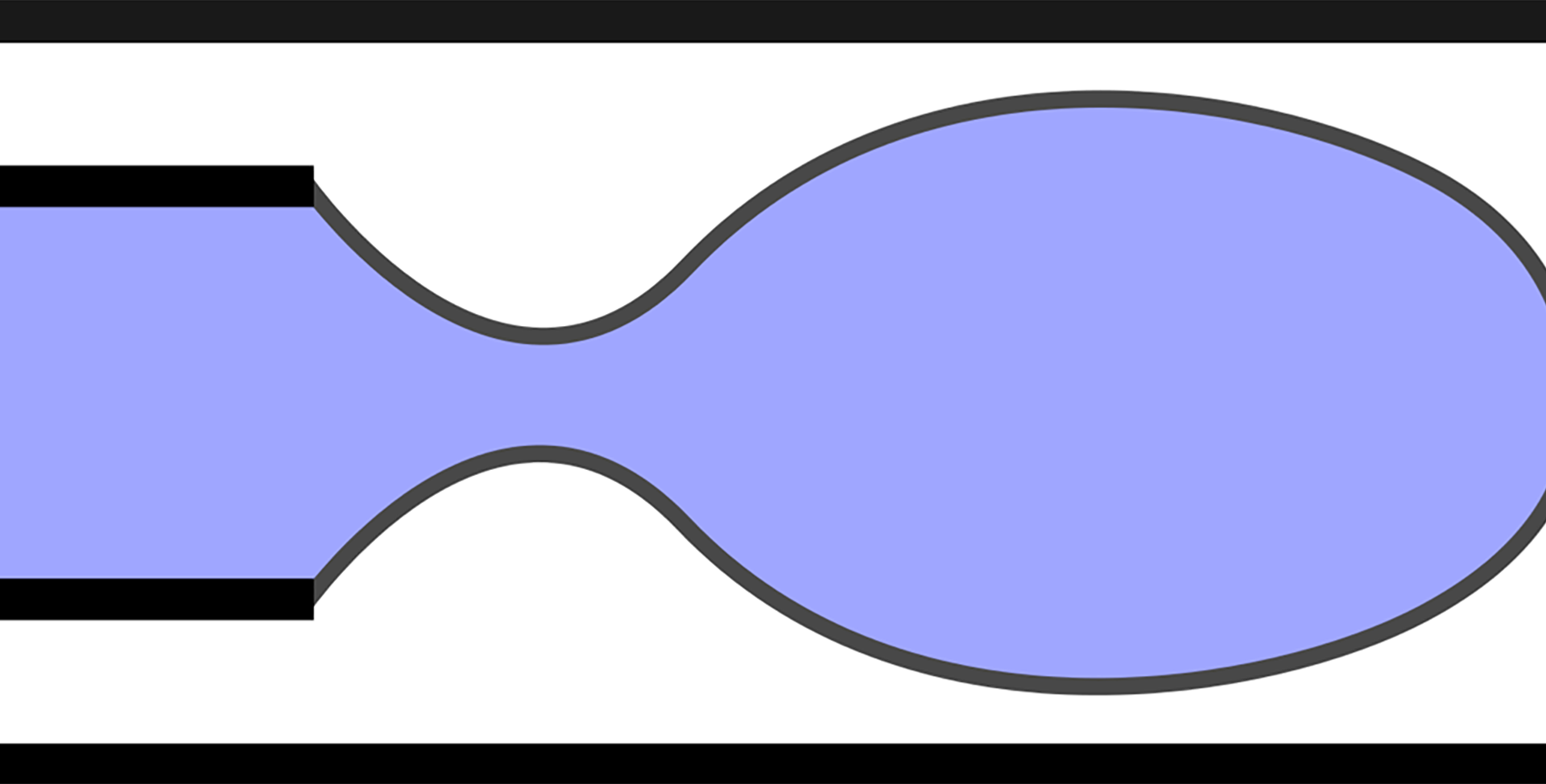
The dynamics of two-fluid capillary flows in channels and pipes underlies numerous applications in biophysics, microfluidics and other industrial processes. Examples include cooling systems and heat exchangers (e.g. Suwankamnerd & Wongwises Reference Suwankamnerd and Wongwises2015; Redo et al. Reference Redo, Jeong, Giannetti, Enoki, Yamaguchi, Saito and Kim2019), aeration within food processing (e.g. Zúñiga & Aguilera Reference Zúñiga and Aguilera2008), biological flows in capillaries (e.g. Kim et al. Reference Kim, Rodriguez, Eldridge and Sackner1986; Ponalagusamy & Selvi Reference Ponalagusamy and Selvi2015) and two-phase flow in porous media (e.g. Wong, Radke & Morris Reference Wong, Radke and Morris1995). Another key application is microfluidic devices designed to generate bubbles, which are used commonly as a contrast agent for ultrasound imaging, and as delivery vehicles in the targeted destruction of tumorous tissues (e.g. Raisinghani & DeMaria Reference Raisinghani and DeMaria2002; Tsutsui, Xie & Porter Reference Tsutsui, Xie and Porter2004; Vladisavljević et al. Reference Vladisavljević, Khalid, Neves, Kuroiwa, Nakajima, Uemura, Ichikawa and Kobayashi2013; Lee et al. Reference Lee, Kim, Han, Lee, Lee, Yoo, Chang and Kim2017). A key aspect of these applications is the control of both the size and frequency of bubbles produced. The most common approach when studying bubble production is experimental investigation (see, for example, review articles by Fu & Ma Reference Fu and Ma2015 and Khan et al. Reference Khan, Ganguli, Edirisinghe and Dalvi2025 and references therein). The analysis presented herein includes, to our knowledge, the first detailed mathematical analysis of bubble pinch-off in the coflow system and the first derivation of an analytical prediction for the pinch-off time from first principles. The study thereby yields a foundation for understanding a key flow regime underlying Taylor bubble formation, yielding both physical insight into how formation is controlled by quasi-static dynamics, and theoretical results that can be used as a basis for testing numerical models and explaining observations. A primary new development of the analysis is to establish a physical and mathematical link connecting pinch-off dynamics in capillaries with quasi-static thin-film modelling, of the kind used widely to describe droplet spreading (Hocking Reference Hocking1982).

Microfluidic devices typically comprise narrow channels of square or rectangular cross-section designed to control the motion, stability and pinch-off of bubbles (e.g. Cubaud et al. Reference Cubaud, Tatineni, Zhong and Ho2005). Their geometries can be tuned in order to produce bubbles of specified size and frequency (e.g. Ma et al. Reference Ma, Zhao, Hou, Huang, Yao, Ding, Wei and Hao2024). Owing to the complexities of many microfluidic geometries and the challenge of modelling the deformable fluid–fluid interface, advancements in the field are often driven by experimental observations, with scaling laws inferred empirically. While there is a variety of microfluidic geometries leading to bubble production, of the most fundamental is coflow, comprising a parallel-walled capillary containing a flowing continuous phase (often a viscous liquid) into which the dispersing phase (typically a gas bubble) is injected via a nozzle placed centrally to the capillary (e.g. Salman, Gavriilidis & Angeli Reference Salman, Gavriilidis and Angeli2006; Utada et al. Reference Utada, Fernandez-Nieves, Stone and Weitz2007; Castro-Hernández et al. Reference Castro-Hernández, Van Hoeve, Lohse and Gordillo2011; Van Hoeve et al. Reference Van Hoeve, Dollet, Gordillo, Versluis, Van Wijngaarden and Lohse2011; Wang et al. Reference Wang, Xie, Lu and Luo2013; Zhang, Li & Thoroddsen Reference Zhang, Li and Thoroddsen2014; Haase Reference Haase2017).

When the injection flux of the bubble is sufficiently larger than that of the liquid phase, elongated capsular bubbles are formed that either completely fill the channel, or have at most a thin fluid film surrounding them (Triplett et al. Reference Triplett, Ghiaasiaan, Abdel-Khalik and Sadowski1999). This regime, known as Taylor bubbles, persists over a wide range of operating conditions and is the most common flow pattern observed for low liquid-to-gas flux ratios (Chen, Kulenovic & Mertz Reference Chen, Kulenovic and Mertz2009). Taylor bubbles possess favourable characteristics such as stable flow patterns and large surface-to-volume ratios for more efficient heat transfer, thus making the production mechanisms of Taylor bubbles a key research problem. Cubaud et al. (Reference Cubaud, Tatineni, Zhong and Ho2005) experimentally investigated the formation of Taylor bubbles in a cross-flow geometry comprising microchannels of square cross-section and proposed an empirical scaling law relating the length of the bubble to the ratio of the gas and liquid flow rates. A similar linear relationship has been confirmed across a range of geometries including flow-focusing devices (Garstecki et al. Reference Garstecki, Stone and Whitesides2005b
; Jensen, Stone & Bruus Reference Jensen, Stone and Bruus2006) and simple coflow geometries (Salman et al. Reference Salman, Gavriilidis and Angeli2006; Xiong, Bai & Chung Reference Xiong, Bai and Chung2007). To date, there has been no theoretical explanation of a law of this kind, including for the most idealised cases of either two-dimensional or axisymmetric coflow.

A pinch-off phenomenon in capillaries that has received particular theoretical attention to date is that which arises in an unforced manner from the Rayleigh–Plateau instability of fluid films coating the interior of an axisymmetric capillary tube (e.g. Goren Reference Goren1962; Everett & Haynes Reference Everett and Haynes1972; Hammond Reference Hammond1983; Frenkel et al. Reference Frenkel, Babchin, Levich, Shlang and Sivashinsky1987; Gauglitz & Radke Reference Gauglitz and Radke1988; Kerchman Reference Kerchman1995; Camassa & Ogrosky Reference Camassa and Ogrosky2015). The azimuthal (hoop) curvature of the coating film generates a positive feedback whereby the driving surface tension increases as the azimuthal radius of curvature narrows. The resulting instability generates a regular periodic pattern of crests and troughs in the lining film that grow and can ultimately connect at the centre of the capillary. This problem was first considered theoretically by Hammond (Reference Hammond1983), specifically addressing the initial growth of the instability using a linear stability analysis with use of lubrication theory. Gauglitz & Radke (Reference Gauglitz and Radke1988) extended the analysis to thicker films by accounting for the full uni-axial axisymmetric shear profile. Integration of the lubrication model allowed for the prediction of the break-up of the fluid film once the thickness grows to the tube centre, with the observation of accelerated thinning prior to pinch-off.

A problem of forced pinch-off was considered by Zhao et al. (Reference Zhao, Pahlavan, Cueto-Felgueroso and Juanes2018) and Pahlavan et al. (Reference Pahlavan, Stone, McKinley and Juanes2019) in which Taylor bubbles are formed by the withdrawal of a viscous fluid, and subsequent displacement by air, in a cylindrical capillary tube. Zhao et al. (Reference Zhao, Pahlavan, Cueto-Felgueroso and Juanes2018) conducted experiments in which a cylindrical tube is initially filled with glycerol that partially wets the capillary. The glycerol is then pulled at a specified flow rate from one end of the tube upon the application of a negative pressure gradient. When the imposed flow rate exceeds a critical value, an air finger forms surrounded by a film of viscous fluid that lines the tube wall. The entrained liquid film recedes, forming a dewetting rim that grows and consequently causes the bubble neck to shrink until pinch-off. It was shown that the pinch-off time was influenced by both the wettability and imposed flow rate. A lubrication model, similar to Gauglitz & Radke (Reference Gauglitz and Radke1988), was used to model the interface, and showed good agreement with the experimentally observed pinch-off profile. Pahlavan et al. (Reference Pahlavan, Stone, McKinley and Juanes2019) presented a detailed mathematical analysis of the lubrication model in the final stages of the pinch-off of an axisymmetric film, showing that the dominance of hoop curvature results in a similarity solution in which the bubble thickness follows a

$1/5$

power-law scaling with time in the final stages prior to pinch-off. This lubrication regime is followed by a linear (non-lubrication) scaling regime very briefly prior to pinch-off.

In summary, theoretical analysis of bubble pinch-off in capillary systems has focused primarily on the natural pinch-off resulting from Rayleigh–Plateau-induced necking, and universal aspects of the form of the solution in the very final stages of axisymmetric pinch-off. However, a detailed mathematical analysis of the full necking evolution in the context of injection-driven pinch-off, as represents the regime of microfluidic bubble generation, has received no detailed theoretical attention. In particular, as noted above, there exists no analysis to explain the experimentally observed scaling laws for bubble pinch-off in the most fundamental problem of coflow, nor more complex geometries.

This paper begins to address this theoretical gap by developing new mathematical and physical understanding in the simplest context of injection-driven bubble pinch-off, where two fluids (one viscous, one inviscid) are injected simultaneously into a planar capillary. The analysis of this idealised configuration, referred to as planar coflow, provides a fundamental system wherein several key aspects of the full necking phenomenon for injection-driven pinch-off can be demonstrated and analysed in detail. The configuration is thus of interest in its own right, as perhaps the simplest model configuration of a capillary flow in which injection-driven pinch-off can occur, and serves as a first step towards addressing more complex axisymmetric and three-dimensional situations with order-unity cross-sectional aspect ratios that typify many microfluidic configurations. A key development here is to introduce the asymptotic framework of quasi-static modelling, commonly used in the analysis of droplet spreading (e.g. Hocking Reference Hocking1982; Kiradjiev, Breward & Griffiths Reference Kiradjiev, Breward and Griffiths2019) to capillary pinch-off, wherein an approximately static interfacial dynamics is coupled to an apparent contact line along a precursor film using asymptotic matching conditions. The regime describes a dominant phase of necking, not limited to the very final stages of pinch-off, providing both new theoretical understanding and a new analytical framework for investigating the pinch-off of Taylor bubbles. Here, we develop the theory, validate it against numerical solutions and use it to develop the first explicit analytical prediction from first principles for the bubble pinch-off frequency in a coflow system.

We begin in § 2 by formulating a lubrication model for the necking disturbance generated in a coflow system based on matching the interface to a downstream extending Taylor bubble. Non-dimensionalisation of the model reveals key underlying intrinsic scales and dimensionless parameters that allow us to systematically characterise the emergent necking dynamics. We conduct a mathematical analysis of the solutions to the lubrication model in § 3, beginning with a demonstration of the pinch-off as the bubble thickness thins to zero, followed by an exploration of the general dependence of the pinch-off time on the dimensionless parameters. The mathematical structure and solutions are reminiscent of those describing injection-driven two-dimensional droplets. Motivated by this observation, we formulate a quasi-static theory for the interfacial evolution, applicable for small capillary numbers, based on coupling a near-static outer region of the necking film with an apparent contact line. Asymptotic analysis of the quasi-static model yields explicit analytical predictions for the pinch-off time, which we validate by comparison with both the lubrication model and full-Stokes simulation. We end the mathematical analysis by evaluating conditions for the self-consistency of the underlying assumptions of the model, namely, that of lubrication theory and of the development of a long (Taylor) bubble into which the necking disturbance spreads. In § 4, we summarise and redimensionalise the key results, discuss limitations of the present study, consider potential new directions and draw qualitative comparisons with the results of prior experimental and numerical studies. We end in § 5 by summarising our main conclusions.

2. Theoretical development

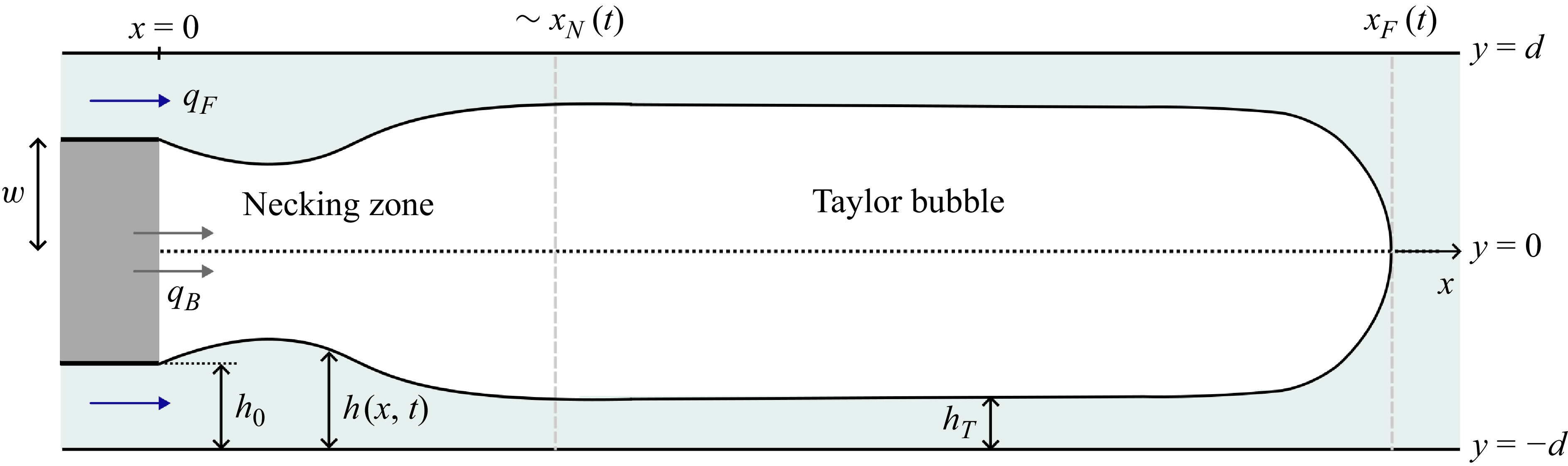
We consider a two-dimensional capillary consisting of parallel rigid boundaries along

$y = \pm d$

, where

$d$

is the half-width of the capillary, assumed uniform (figure 1). The capillary is filled with a viscous fluid of dynamic viscosity

$\mu$

and velocity field

$\boldsymbol u(x,y,t) = (u,v)$

that is introduced at a prescribed volumetric flux per unit width

$2 q_F$

. Interior to the capillary, an inviscid fluid is injected at a constant volumetric flux per unit width

$2q_B$

via an injection nozzle of thickness

$2w$

. The thickness of the fluid film around the bubble is

$h(x,t)$

. The conditions on the film are

(2.1a–b)

\begin{gather} h(0,t) = h_0, \qquad q(0,t) = q_F, \end{gather}

where

$h_0 = d – w$

, such that the interface

$h(x,t)$

is fixed at the nozzle, and

(2.2)

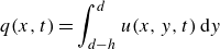
\begin{align} q(x,t) = \int _{d-h}^d u(x,y,t) \; \textrm {d} y \end{align}

is the volumetric flux per unit width of the viscous film. The set-up forms the configuration of coflow, a system that induces periodic pinch-off of the injected inviscid fluid phase (e.g. Ma et al. Reference Ma, Zhao, Hou, Huang, Yao, Ding, Wei and Hao2024). The condition of interface continuity (2.1a
) implies that the interface separates from the walls of the nozzle, a property observed experimentally (e.g. Xiong et al. Reference Xiong, Bai and Chung2007; Lin et al. Reference Lin, Bao, Tu, Yin, Gao and Lin2019; Sontti & Atta Reference Sontti and Atta2019) and similar to pinning conditions used in static and dynamic Young–Laplace problems (e.g. Finn Reference Finn1986), particularly in the context of pendant drops (e.g. Lee & Hwang Reference Lee and Hwang2025) and liquid bridges (e.g. Meseguer, Slobozhanin & Perales Reference Meseguer, Slobozhanin and Perales1995).

Figure 1.

Schematic representing the asymptotic structure of a developing Taylor bubble formed by injection via a nozzle. The flow structure can be divided into two regions: (i) the necking region where the fluid film thickens locally in the vicinity of the input nozzle, and (ii) the Taylor bubble region comprising an approximately circular front connected to a region of near uniform film thickness.

The development of Taylor bubbles is a dominant flow pattern and has been studied experimentally in a range of geometries including circular capillaries (e.g. Salman et al. Reference Salman, Gavriilidis and Angeli2006; Zhao et al. Reference Zhao, Pahlavan, Cueto-Felgueroso and Juanes2018) and microchannels of square cross-section (e.g. Cubaud et al. Reference Cubaud, Tatineni, Zhong and Ho2005; Lu et al. Reference Lu, Fu, Zhu, Ma and Li2016; Huang & Yao Reference Huang and Yao2022; Sun et al. Reference Sun, Dang, Jia, Shen and Liu2025). In this regime, elongated capsular bubbles form that are separated by liquid slugs. As a result of the development of stagnant flow interior to the developing Taylor bubble, a region of localised thinning forms a neck near the orifice. The neck proceeds to thicken, eventually instigating pinch-off. Repetition of this process ultimately generates a train of Taylor bubbles.

Motivated by this observed flow structure, we consider the configuration in two regions: a necking zone, residing in

$0 \leqslant x \lesssim x_N(t)$

, where

$x_N(t)$

is the characteristic scale of the developing necking disturbance at time

$t$

; and the extending Taylor bubble, lying in the region

$x_N(t) \lesssim x \leqslant x_F(t)$

, where

$x_F(t)$

is the position of the bubble cap (figure 1). The characteristic size of the necking disturbance,

$x_N(t)$

, is not known a priori and will, in general, grow with time. The development of a long (Taylor) bubble assumed in this asymptotic structure (as opposed to smaller bubbles, as is more characteristic when the film flux is larger than the bubble flux (Triplett et al. Reference Triplett, Ghiaasiaan, Abdel-Khalik and Sadowski1999)) requires the bubble cap to lie further ahead of the length scale of the necking disturbance

(2.3)

\begin{equation} x_N(t) \ll x_F(t). \end{equation}

If the condition above applies, then the front of the bubble extends beyond the necking disturbance, a structure indicated both experimentally and by numerical simulations of Taylor bubble formation (e.g. Cubaud et al. Reference Cubaud, Tatineni, Zhong and Ho2005; Salman et al. Reference Salman, Gavriilidis and Angeli2006; Xiong et al. Reference Xiong, Bai and Chung2007; Chen et al. Reference Chen, Kulenovic and Mertz2009; Dang, Yue & Chen Reference Dang, Yue and Chen2015; Mei et al. Reference Mei, Le Men, Loubière, Hébrard and Dietrich2022). Thus, the necking disturbance grows into the uniform-thickness interior of the Taylor bubble. The self-consistency of the condition (2.3) will be evaluated a posteriori, with the finding that, as anticipated based on experimental observations for qualitatively similar configurations (Triplett et al. Reference Triplett, Ghiaasiaan, Abdel-Khalik and Sadowski1999), it is indeed directly based on the flux ratio

$q_F/q_B$

(§ 3.3). In developing our model for the necking film, we consider the Taylor bubble and necking-zone regions in turn, before connecting the two regions with a matching condition.

2.1. The Taylor bubble

The Taylor bubble in general comprises a capsular structure with a round cap connected to a region of approximately uniform thickness in its interior (figure 1). The control of the film thickness in the uniform region,

$h_T$

, has received significant attention since it was considered experimentally by Fairbrother & Stubbs (Reference Fairbrother and Stubbs1935) and Taylor (Reference Taylor1961), and theoretically by Bretherton (Reference Bretherton1961). Bretherton (Reference Bretherton1961) shows that the relative size of

$h_T$

depends crucially on the magnitude of the capillary number

(2.4)

\begin{equation} C = \frac {\mu q_B}{\gamma d}, \end{equation}

representing the ratio of the size of viscous stresses to the size of capillary stresses on the scale of the capillary width

$d$

. For small

$C$

, Bretherton (Reference Bretherton1961) demonstrates an asymptotic structure defined by a frontal cap, with a leading-order circular cross-section dominated by surface tension, that is matched to the long interior of the inviscid bubble, where the exterior film is stagnant, through a region in which lubrication theory is applied. Analysis of this structure in the context of steady travelling-wave states yields the analytical expression for the film thickness in the approximately horizontal region

(2.5)

\begin{equation} h_T \sim 1.3375\, \left ( \frac {\mu q_B}{\gamma d} \right )^{2/3} d \equiv 1.3375 \, C^{2/3} d \qquad (C \to 0), \end{equation}

implying a control by a combination of viscous, capillary and geometric parameters.

For moderate to large

$C$

, viscous stresses play an important role at the bubble cap, and a full-Stokes resolution is necessary there. In general, the interior thickness of the Taylor bubble satisfies

(2.6)

\begin{equation} h_T = B(C) d, \end{equation}

where

$B(C)$

is a dimensionless function of

$C$

only (figure 2), with the property that

$B(C) \sim 1.3375 \, C^{2/3}$

as

$C \to 0$

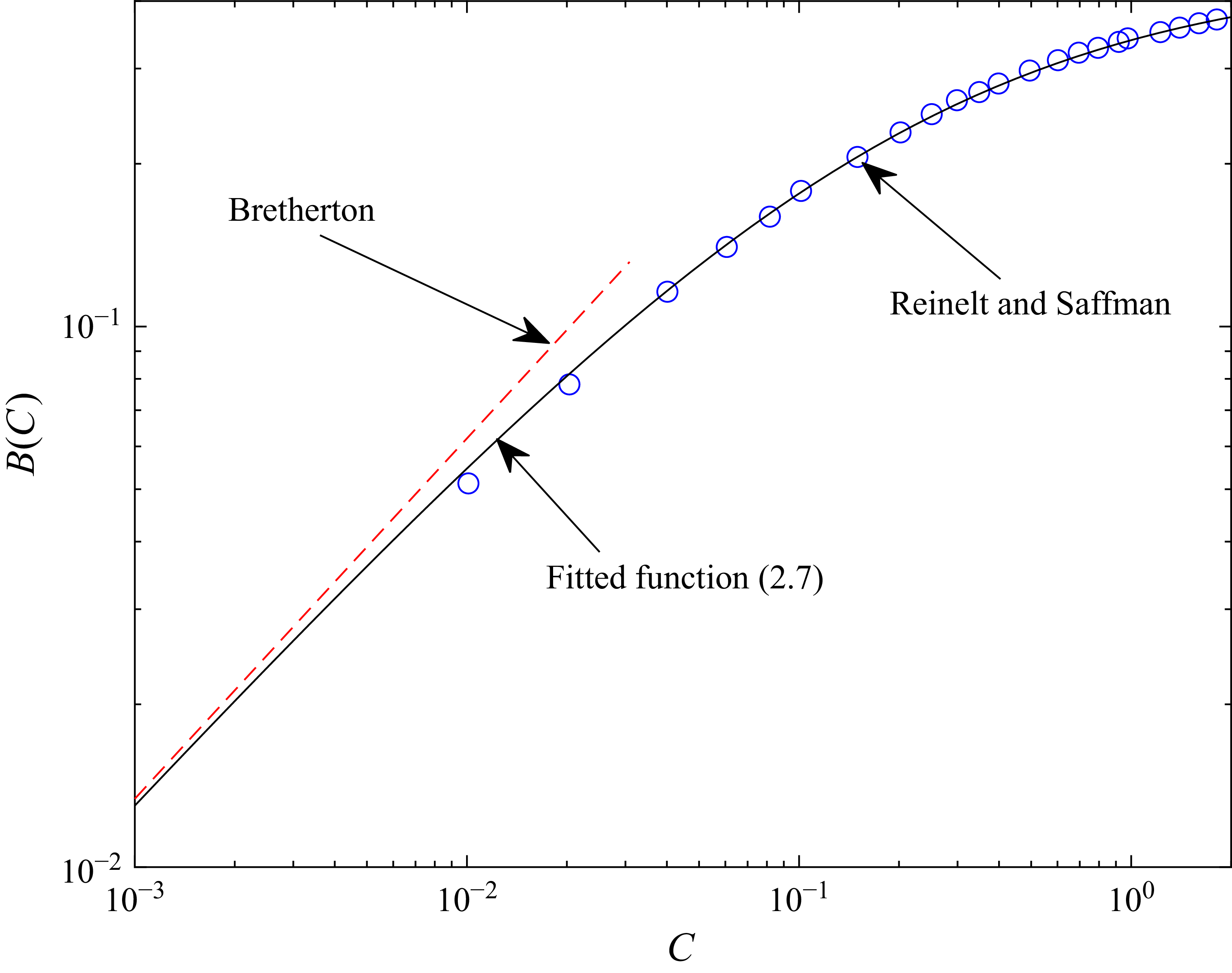
in conformity with (2.5). Full-Stokes numerical solutions (Reinelt & Saffman Reference Reinelt and Saffman1985) for two-dimensional Taylor bubbles have determined

$B(C)$

over a broad range of

$C$

for

$C \gtrsim 10^{-2}$

(circular markers). For sufficiently large

$C$

, capillary stresses ultimately become negligible compared with viscous stresses, and the interior thickness saturates towards a factor multiple of the capillary width,

$h_T \sim 0.45\, d$

. We note that the analytical function

(2.7)

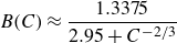
\begin{equation} B(C) \approx \frac {1.3375}{2.95 + C^{-2/3}} \end{equation}

provides a good representation (black, solid curve in figure 2) that captures both the small-

$C$

limiting result of Bretherton (2.5) (red, dashed) and the moderate- to large-

$C$

values determined numerically by Reinelt & Saffman (Reference Reinelt and Saffman1985).

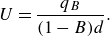
Mass conservation in the travelling-wave state implies that the constant translation speed of the bubble cap is given by (Bretherton Reference Bretherton1961)

(2.8)

\begin{equation} U = \frac {q_B}{(1 – B)d}. \end{equation}

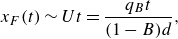
With

$t$

representing the time since the injection is initiated, the leading-order position of the bubble nose can be characterised by

(2.9)

\begin{equation} x_F(t) \sim Ut = \frac {q_Bt}{(1-B)d}, \end{equation}

or simply

$x_F \sim (q_B/d) t$

in the limit of

$B \to 0$

arising for

$C \to 0$

.

Figure 2.

The empirical expression for the universal function

$B(C) \equiv h_T/d$

defining the size of the interior thickness of the Taylor bubble

$h_T$

to the capillary half-width, defined by (2.6). The numerical results of Reinelt & Saffman (Reference Reinelt and Saffman1985) are shown as blue circular markers. The small-

$C$

result of Bretherton (Reference Bretherton1961) is shown as a red dashed line. The fitted analytical function (2.7) is shown as a solid black curve.

2.2. The necking zone

We define the necking zone as lying between the injection nozzle and the interior of the Taylor bubble,

$0 \leqslant x \lesssim x_N(t)$

(figure 1), where

$x_N(t)$

is a time-dependent characteristic scale of the developing necking disturbance to be predicted. Within the necking zone, the viscous film squeezes the Taylor bubble, instigating pinch-off.

In modelling the necking interface, we apply lubrication theory, based formally on the requirement that the interfacial gradient in this region is small

(2.10)

\begin{equation} h_x \ll 1. \end{equation}

Satisfaction of lubrication theory in the necking zone is not obvious a priori because the magnitude of the interfacial gradient

$h_x$

is dependent on the relative longitudinal and transverse length scales of the resulting solution, as characterised by the aspect ratio

$\sim h_m(t)/x_N(t)$

, where

$h_m(t)$

is the maximal film thickness

(2.11)

\begin{equation} h_m(t) = \max _{x} \left ( h(x,t) \right )\!. \end{equation}

We follow the asymptotic heuristic of adopting lubrication theory and assess the self-consistency of its predictions in maintaining

$h_x \ll 1$

within the necking zone a posteriori.

Lubrication theory is used extensively in modelling capillary flows. Examples include liquid film breakup in capillary tubes driven by the Rayleigh–Plateau instability (e.g. Hammond Reference Hammond1983; Gauglitz & Radke Reference Gauglitz and Radke1988; Rykner et al. Reference Rykner, Saikali, Bruneton, Mathieu and Nikolayev2024), two-phase fluid displacement in capillaries (e.g. Bretherton Reference Bretherton1961; Zhao et al. Reference Zhao, Pahlavan, Cueto-Felgueroso and Juanes2018; Pahlavan et al. Reference Pahlavan, Stone, McKinley and Juanes2019; Lu, Li & Gao Reference Lu, Li and Gao2023), coating (e.g. Landau & Levich Reference Landau and Levich1942; Eggers Reference Eggers2004, Reference Eggers2005; Snoeijer et al. Reference Snoeijer, Andreotti, Delon and Fermigier2007; Gao et al. Reference Gao, Li, Feng, Ding and Lu2016) and capillary-driven droplets (e.g. Hocking Reference Hocking1983; King & Bowen Reference King and Bowen2001; Savva & Kalliadasis Reference Savva and Kalliadasis2009; Kiradjiev et al. Reference Kiradjiev, Breward and Griffiths2019). The governing equations of lubrication theory are

(2.12a–b)

\begin{gather} \mu u_{yy} = p_x, \qquad p_y = 0, \end{gather}

where

$u(x,y,t)$

is the longitudinal velocity of the viscous fluid,

$p(x,y,t)$

is the pressure field of the viscous fluid and we use subscripts to denote partial derivatives. With

$\kappa = h_{\textit{xx}}$

representing the linearised interfacial curvature, and

$\gamma$

the interfacial coefficient of surface tension, the interface is subject to the following conditions on the capillary wall,

$y=d$

, and bubble interface,

$y = d-h(x,t)$

:

(2.13a–c)

\begin{gather} u(x,d,t) = 0, \qquad u_y(x,d-h,t) = 0, \qquad [p]_{y =(d-h)_{-}}^{y = (d-h)_+} = -\gamma \kappa , \end{gather}

representing conditions of no slip on the sides of the capillary, no stress at the interface with the inviscid bubble and the jump in capillary stress across the interface, respectively. Integrating (2.12b
) subject to the jump condition (2.13c
), we obtain the pressure in the film

(2.14)

\begin{equation} p(x,t) = p_0 – \gamma \kappa (x,t), \end{equation}

where

$p_0$

is an arbitrary constant reference pressure; owing to the assumed incompressibility of the fluids,

$p_0$

will have no effect on the dynamics of the problem. Integrating (2.12a
) twice and applying (2.13a
,
b
), we obtain the velocity profile

(2.15)

\begin{equation} u=\frac {p_x}{2\mu }(y-d)(y-d+2h), \end{equation}

and hence, with (2.13c
) and

$\kappa = h_{\textit{xx}}$

, the volume flux (per unit width)

(2.16)

\begin{equation} q(x,t) = \int _{d-h}^{d} u \; \textrm {d} {y} = \frac {\gamma }{3\mu } h^3 h_{\textit{xxx}}. \end{equation}

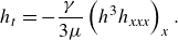
Substituting the above into the continuity equation of the fluid film,

$h_t = -q_x$

, we obtain the governing nonlinear hyperdiffusion equation

(2.17)

\begin{equation} h_t = -\frac {\gamma }{3\mu } \left (h^3 {h}_{\textit{xxx}}\right )_x. \end{equation}

Conditions (2.1) provide the two boundary conditions at the input nozzle

(2.18)

\begin{equation} h(0,t) = h_0, \qquad q(0,t) = q_F. \end{equation}

We couple the necking film to the interior thickness of the Taylor bubble (2.6) by applying the matching condition

(2.19)

\begin{equation} \lim _{x \to \infty } h = h_T, \end{equation}

which creates a connection between the dynamics of the necking zone and the interior thickness of the film within the Taylor bubble

$h_T$

. For conformity with (2.19), we apply the initial condition

(2.20)

\begin{equation} h(x,0) = h_T. \end{equation}

Equations (2.17)–(2.20) form a closed system describing the growth of the necking film

$h(x,t)$

. At the critical time

$t_*$

defined by

(2.21)

\begin{equation} h_m(t_*) \equiv \max _{x} \left ( h(x,t_*) \right ) = d, \end{equation}

the viscous fluid spans the width of the channel, defining the pinch-off time of the bubble. In the confined planar configuration considered in this paper, we will find that the fluid film grows locally in the necking region independently on either side of the channel centreline until a point where the two fluid films meet and the bubble thickness becomes zero in finite time

$t_*$

. Our focus will be on understanding the parametric control of the pinch-off time

$t_*$

.

2.3. Dimensionless system

In order to maximally reduce the parametric dependence of the model (2.17)–(2.20), we define the following non-dimensional variables based on intrinsic scales:

(2.22)

\begin{equation} x = \left ( \frac {\gamma h_T^4}{ \mu q_F } \right )^{1/3} \hat {x} , \qquad t = \left ( \frac {\gamma h_T^7}{\mu q_F^4} \right )^{1/3} \hat {t}, \qquad h = h_T \hat {h}. \end{equation}

Upon dropping hats, (2.17) becomes

(2.23)

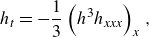
\begin{equation} h_t = -\frac {1}{3}\left (h^3h_{\textit{xxx}}\right )_x, \end{equation}

with dimensionless flux

$q=({1}/{3})h^3h_{\textit{xxx}}$

. Conditions (2.18) and (2.19) become

(2.24a-c)

\begin{gather} h(0,t) = \frac {H}{B}, \qquad q(0,t) = 1, \qquad \lim _{x\to \infty }h=1, \end{gather}

where

$H = h_0/d$

and

$B = h_T/d$

. The initial condition (2.20) becomes

(2.25)

\begin{equation} h(x,0) = 1, \end{equation}

and the pinch-off criterion (2.21) is

(2.26)

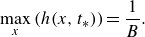
\begin{equation} \max _{x} \left ( h(x,t_*) \right ) = \frac {1}{B}. \end{equation}

The non-dimensionalisation has reduced the dependence of the solutions to two dimensionless numbers

(2.27)

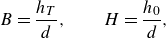
\begin{equation} B = \frac {h_T}{d}, \qquad H = \frac {h_0}{d}, \end{equation}

representing the ratio of the interior film thickness

$h_T$

to the half-width of the capillary

$d$

, and the ratio of the film thickness at the inlet to the half-width of the capillary, respectively. The number

$B$

is correspondent with the quantity

$B(C)$

given by the one-to-one function of

$C$

represented by (2.7), and is thus a surrogate for the capillary number. Capillary numbers in microfluidic systems, for example, are characteristically small (e.g. Anna Reference Anna2016) with

$C \lesssim 10^{-2}$

, for which (2.7) gives

$B \lesssim 0.1$

. The second dimensionless number

$H$

sets the level of confinement of the nozzle relative to the width of the capillary. The number is restricted to

$0 \lt H\lt 1$

, with

$H \ll 1$

representing a strongly confining nozzle.

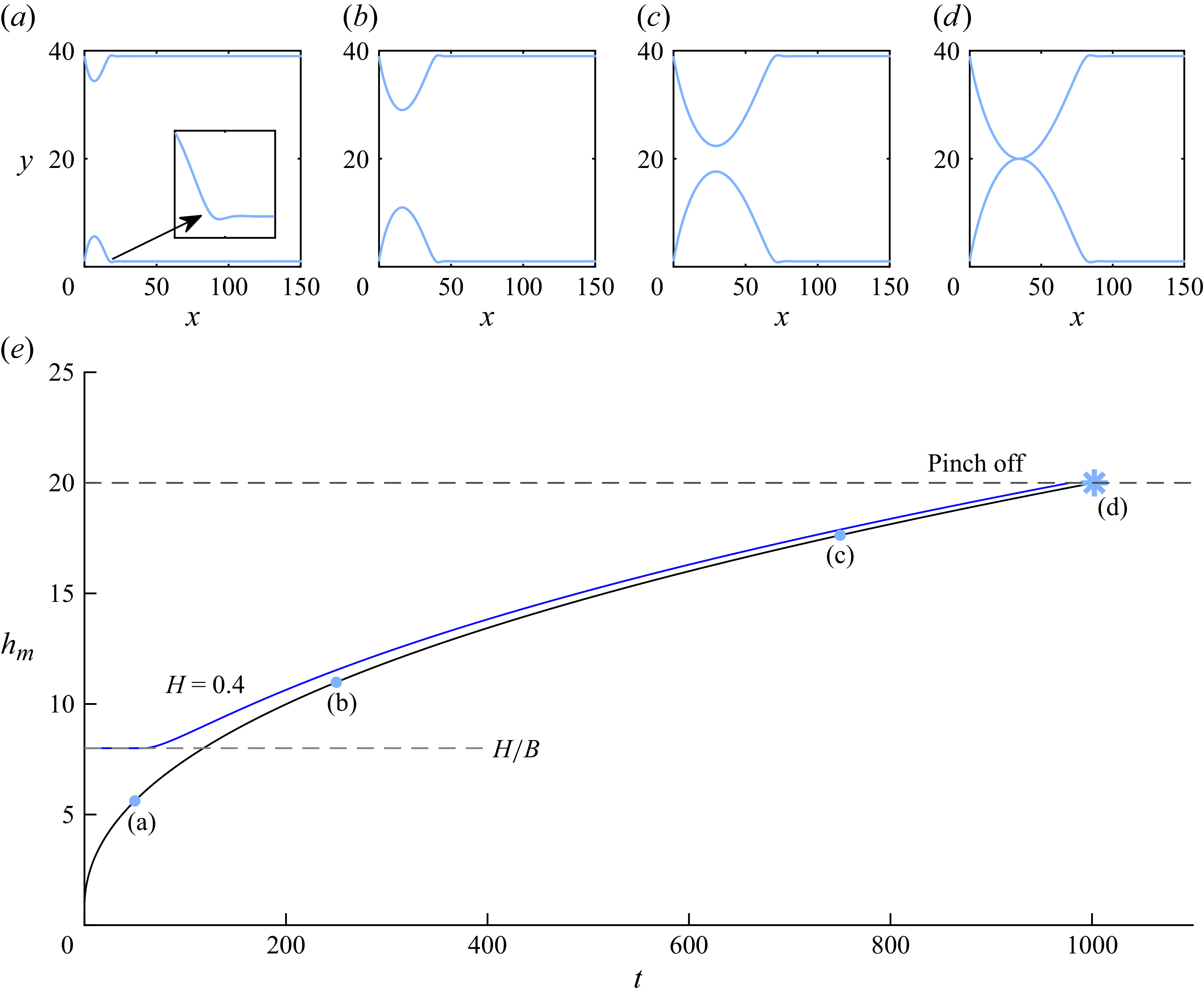
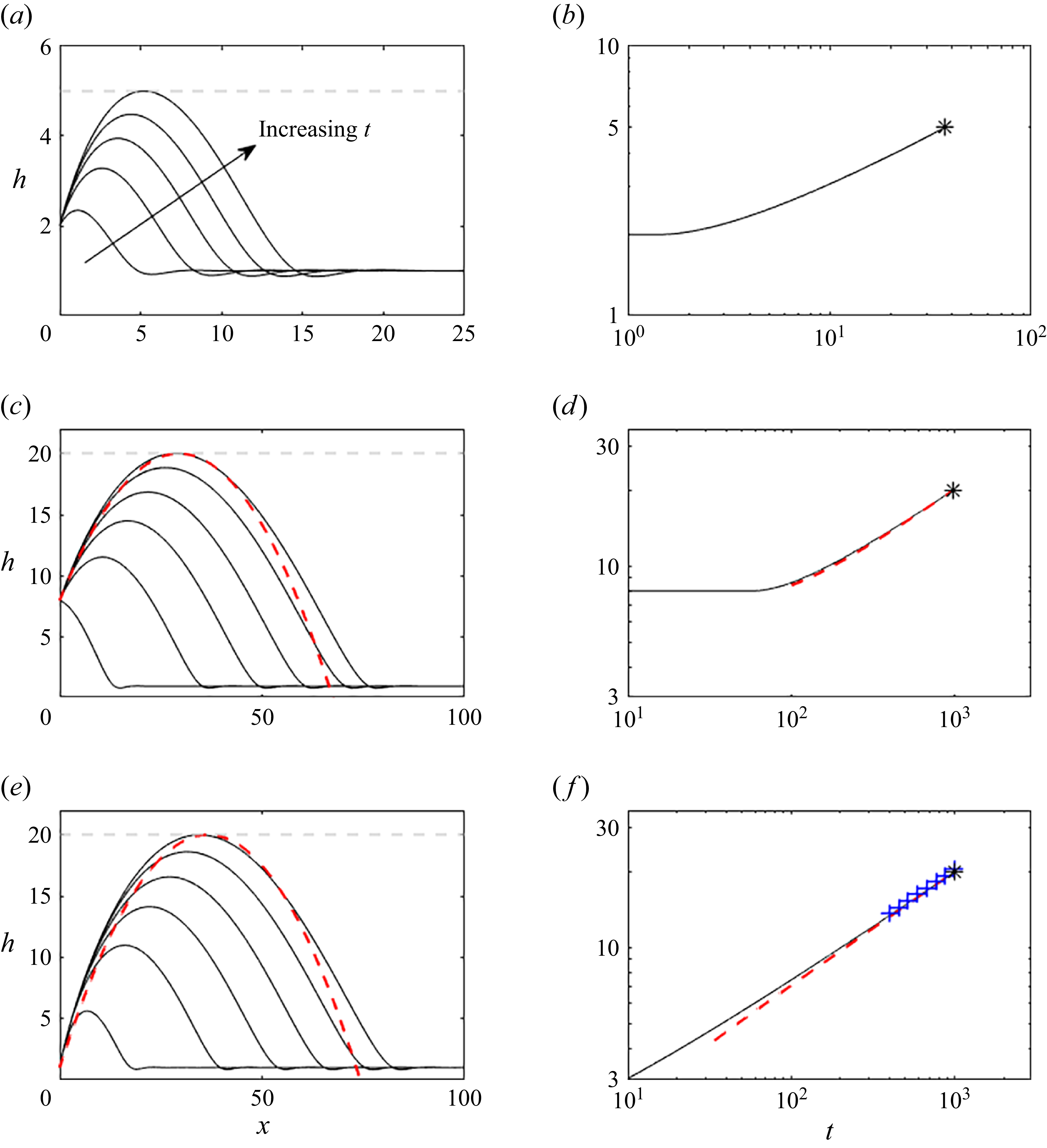
Figure 4.

Numerical solutions to the time-dependent necking-zone model (2.23)–(2.25) (black) for

$(a)$

$B=0.2$

and

$H=0.4$

at

$t=4,12,20,28,t_*\approx 37.09$

,

$(c)$

$B=0.05$

and

$H=0.4$

at

$t=50,250,450,650,850$

,

$t_*\approx 978.35$

and

$(e)$

$B=0.05$

and

$H=0.05$

at

$t=50,250,450,650,$

$850,t_*\approx 1002.3$

. The red dashed line represents the parabola (3.4) at final time

$ t_*$

. The centreline of the channel, representing the thickness of the film at which pinch-off occurs,

$h_m(t_*) = 1/B$

, is indicated by a horizontal dashed grey line in the (a,c,e). The panels on the right plot the corresponding maximal film thickness

$h_m$

as a function of time

$ t$

, showing approach to a quasi-static solution with front position given by (3.14) (red dashed). The asymptotic prediction for

$h_m(t)$

for the small-

$H$

limit (3.21) is overlayed as blue crosses in the case

$H=0.05$

.

3. Mathematical analysis

An illustrative solution to the system (2.23)–(2.25) is shown in figure 3 for

$B=0.05$

and

$H=0.05$

. The solution was obtained numerically using the method of lines, in which spatial derivatives are discretised using centred differences and time stepping is conducted using the stiff MATLAB integrator ode15s. The top four panels show snapshots of the interface evolution at the progression of times

$t=50,250,750$

up to a critical time of pinch-off,

$t_* \approx 1002$

, illustrating the development of a near-parabolic necking disturbance. The near-parabolic region transitions to the downstream region of uniform thickness relatively abruptly through a region in which the interface exhibits a small-scale spatial oscillation (shown in a zoomed inset of panel a). Since the fluid is effectively stationary in the thin film of uniform thickness that surrounds the bubble, subsequent injection amasses fluid at the injection nozzle which causes the surrounding film thickness to swell and ultimately results in pinch-off of a bubble. The lower panel presents the evolution of the maximal film thickness

$h_m(t)$

, showing that it grows with a sublinear trend before attaining the pinch-off value

$h_m(t_*) = 1/B$

, indicated by a horizontal dashed line, at

$t_* \approx 1002$

. The evolution of the maximal thickness

$h_m(t)$

for

$H=0.4$

is shown in blue, exhibiting a brief phase where the thickness of the film at the nozzle represents the maximum thickness

$h_m = H/B$

(prior to the formation of a turning point in the interface) up to

$t \approx 60$

, and a slightly faster pinch-off time of

$t_* \approx 978$

relative to the case of a larger nozzle.

Figure 4 shows further illustrative solutions for

$(a)$

$B=0.2$

and

$H=0.4$

,

$(c)$

$B=0.05$

and

$H=0.4$

and

$(e)$

$B=0.05$

and

$H=0.05$

, with the interface evolution shown on the left and the evolution of the maximal thickness shown on the right as a solid black curve. In each case, the disturbance retains a qualitatively parabolic form, and grows until the point of pinch-off

$h_m(t_*) = 1/B$

, represented by a grey dashed horizontal line in the left-hand panels and an asterisk in the right-hand panels. Comparing cases (

$a$

) and (

$c$

), we see that smaller

$B$

results in a longer time to pinch-off, with the magnitude and longitudinal scale of the oscillation at the front of the spreading region being comparatively smaller. The bottom case (

$e$

) shows the same case as (

$c$

) but with a nozzle that spans the majority of the capillary

$(H=0.05)$

.

To determine the pinch-off time

$ t _*(H,B)$

over a continuous range of

$B$

for a given value of

$H$

, we begin by solving (2.23)–(2.25) numerically for the evolving interface profile

$h(x, t )$

. We then read off the time

$ t _*$

at which

$h_m( t _*) = 1/B$

over a range of

$B$

. The determined function

$ t _*(H,B)$

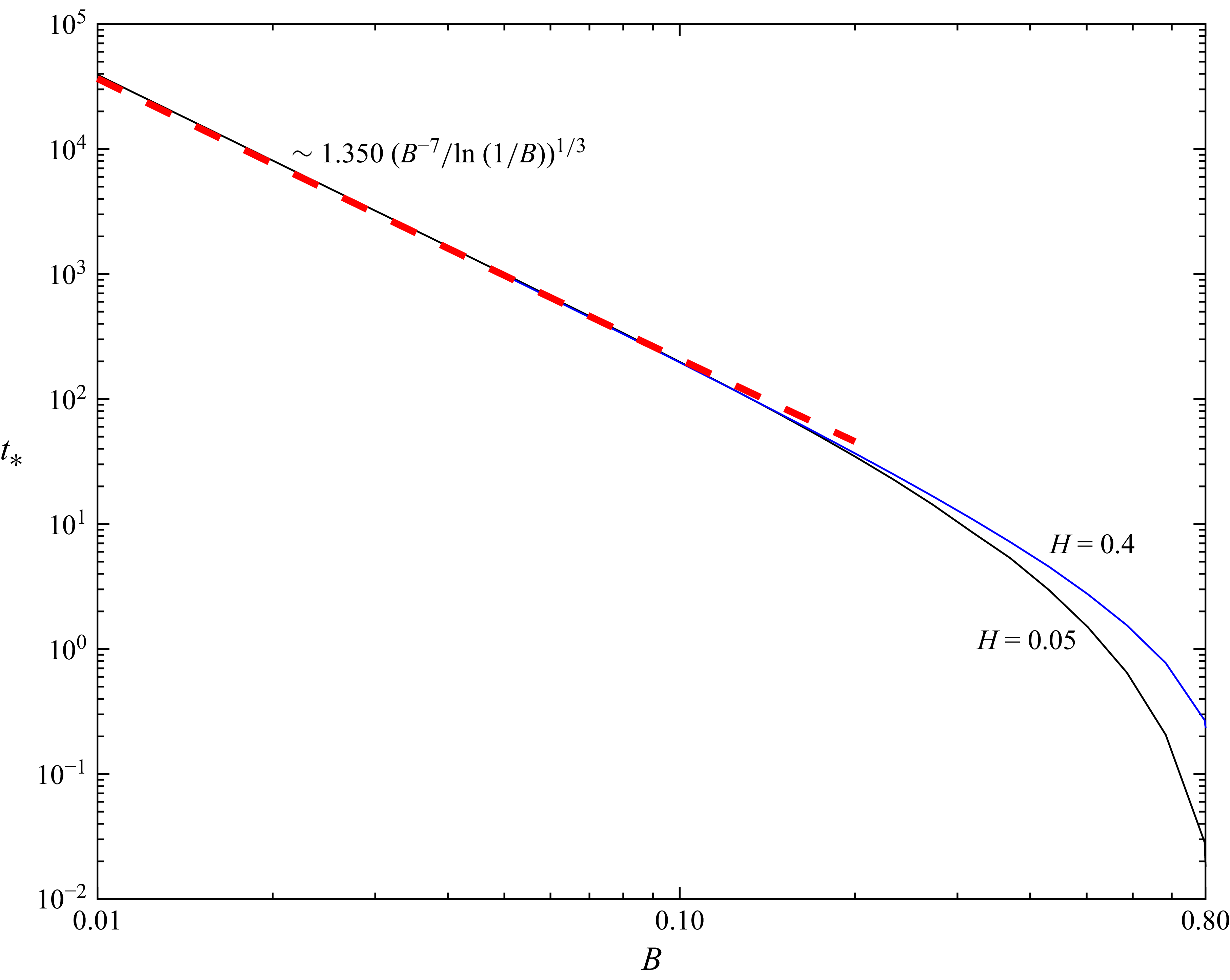
, representing the time of pinch-off over the full parameter space of the necking-zone theory, is shown as a function of

$B$

in figure 5 for two illustrative values of

$H = 0.05$

and 0.4. The function

$ t _*$

generally forms a decreasing function of the film thickness

$B$

, appearing to converge to an approximately

$B^{-7/3}$

asymptotic trend as

$B \to 0$

. At moderate values of

$B \gtrsim 0.3$

, we see that the effect of the nozzle–wall spacing

$H$

can significantly impact the pinch-off time by a factor of

$2$

–3. For small

$B \lesssim 0.1$

, the pinch-off times appear to become insensitive to the nozzle–wall spacing

$H$

, with both example values of

$H$

approaching a mutual asymptote as

$B \to 0$

. The determination of

$t_* (B,H)$

, when combined with the intrinsic scales used for non-dimensionalisation (2.22), yields a general functional dependence of the pinch-off time of the Taylor bubble in the two-dimensional coflow system. The results demonstrate the emergence of a simple asymptotic trend in the dependence of

$t_*$

on

$B$

in the key limit of

$B \lesssim 0.1$

, which we now seek to understand.

3.1. Quasi-static theory

We formulate a simplified analytical theory based on utilising an asymptotic framework of quasi-static interfacial evolution. A theoretical approach of this kind has been applied previously, in particular, in the context of droplet spreading (e.g. Hocking & Rivers Reference Hocking and Rivers1982; Hocking Reference Hocking1983; King & Bowen Reference King and Bowen2001; Savva & Kalliadasis Reference Savva and Kalliadasis2009, Reference Savva and Kalliadasis2011; Vellingiri, Savva & Kalliadasis Reference Vellingiri, Savva and Kalliadasis2011; Savva & Kalliadasis Reference Savva and Kalliadasis2013; Kiradjiev et al. Reference Kiradjiev, Breward and Griffiths2019). The theory, applicable for small capillary number (equivalently

$B \ll 1$

), is based on a separation of the flow into two asymptotic zones: an outer region, wherein a fast diffusive time scale maintains the interface close to the shape of a static meniscus (a parabola for two-dimensional droplets; Kiradjiev et al. Reference Kiradjiev, Breward and Griffiths2019); and an inner zone localised near a frontal apparent contact-line position, wherein the flow is matched to the precursor film. The outer region evolves quasi-statically in response to a slow time scale associated with the evolution of the contact line. The leading-order equation of the outer region is the Young–Laplace equation describing a static meniscus subject to the condition that the interface connects to the contact-line position. The inner zone instead forms a travelling-wave state (exhibiting the small spatial oscillation in the interface of the kind we see in figure 3
a), the solution of which yields a matching condition (the Cox–Voinov law; Voinov Reference Voinov1976; Cox Reference Cox1986) on the outer region.

In the present context, we can interpret the necking dynamics as a kind of forced droplet-like disturbance that spreads into an effective precursor film left by the extending Taylor bubble. As noted above, a quasi-static theory requires the necking disturbance to grow much thicker than the precursor film. In our context, we recall that the dimensionless precursor-film thickness is unity and the pinch-off criterion is

$h_m(t_*) = 1/B$

. Therefore, if

$B \ll 1$

, the necking disturbance will necessarily grow much thicker than the precursor film prior to pinch-off, with

$1 \ll h_m(t) \leqslant 1/B$

. A quasi-static dynamics can therefore be anticipated to arise for

$B \ll 1$

over the ‘large’ temporal range

$1 \ll t \leqslant t_*(H,B)$

. Within this dominant time interval, the necking disturbance, in accordance with the proposed quasi-static theory, forms a two-zone structure: an outer quasi-static zone of approximately parabolic form; and an inner zone localised near an apparent contact line

$ x _N( t )$

that advances in accordance with a Cox–Voinov law. We proceed to develop the quasi-static theory and compare its predictions with the full time-dependent theory.

We begin by solving for the outer quasi-static region. Within the quasi-static framework, the flow adjusts rapidly to a near-static state with

$q \approx 0$

and hence, from the expression for flux

$q = ({1}/{3}) h^3 h_{\textit{xxx}}$

given below (2.23),

(3.1)

\begin{equation} h_{\textit{xxx}} \approx 0. \end{equation}

The above represents the equation describing the ultimate shape formed by relaxation under linearised surface tension,

$\kappa _x =0$

; in other words, it is the linearised Young–Laplace equation describing a static two-dimensional meniscus. On the scales of the quasi-static outer region (

$h \gg 1$

), the precursor-film thickness is effectively vanishing to leading order,

(3.2)

\begin{equation} h( x _N( t ), t ) = 0. \end{equation}

The condition at the input nozzle (2.24) gives the further boundary condition

(3.3)

\begin{equation} h(0, t ) = H/B. \end{equation}

Integration of (3.1) subject to (3.2) and (3.3) gives us the parabola

(3.4)

\begin{equation} h(x,t) = \left ( A( t ) x +\frac {H}{Bx_N(t)} \right ) (x_N(t) – x), \end{equation}

where

$A( t )$

is a constant of integration related to the height of the parabola. Since the volume must equal

$ t$

in accordance with the dimensionless input flux

$q(0, t )=1$

, the interface must satisfy the volume constraint

(3.5)

\begin{equation} \int _0^{ x _N} h \; \textrm {d} { x } = \frac {1}{6}A(t) x _N^3+\frac {H}{2B}x_N = t , \end{equation}

where we have substituted (3.4) and evaluated the integral. Hence,

(3.6)

\begin{equation} A( t ) = \frac {3}{x_N(t)^{3} } \left ( 2 t – \frac {Hx_N( t )}{B} \right )\!. \end{equation}

The only remaining unknown in the quasi-static solution (3.4) is now the position of the contact line

$ x _N(t)$

. Thus, we require a further condition for closure.

The additional condition is given by a Cox–Voinov relation that matches the quasi-static solution to the precursor film via an inner travelling-wave state in the vicinity of

$x \approx x_N(t)$

. Within the inner region, the solution transitions from its approximately linear form predicted by the outer solution (3.4) as

$ x \to x _N( t )$

to the downstream precursor-film thickness. A step-by-step derivation of the associated matching condition

(3.7)

\begin{equation} h_x^3 = -3\dot {x}_N\ln \left(\dot {x}_Nx_N^3\right) \qquad \big(x = x_N(t) \big), \end{equation}

reviewing its development from (2.23), is provided in Appendix A. The result relates the rate of advancement of the contact line

$\dot x_N(t)$

to the instantaneous interfacial gradient of the outer solution at the contact line

$h_x(x_N,t)$

. The length scale of the inner zone is of order

$\sim (\dot x_N)^{-1/3}$

, and hence it is necessary that

$(\dot x_N)^{-1/3} \ll x_N$

in order for the required length-scale separation defining the quasi-static regime to apply. In other words, the argument of the natural logarithm in (3.7) is intrinsically large as part of the consistency of the theory. As

$x_N(t)$

grows, the condition

$(\dot x_N)^{-1/3} \ll x_N$

will become ever more strongly satisfied with time (

$t \gg 1$

), concurrently with the thickness becoming much larger than that of the precursor film,

$h_m(t) \gg 1$

. The control of

$x_N(t)$

implied by the matching condition (3.7) is solely responsible for introducing dependences of the quasi-static evolution on the viscous and capillary parameters.

With the system now fully closed, we seek an explicit evolution equation for the contact-line position

$x_N(t)$

. First, we isolate the rate of change

$\dot x_N(t)$

in (3.7) by writing that equation in the equivalent form

(3.8)

\begin{equation} x_N^3 \dot {x}_N = \exp \left (W\left (- \frac {1}{3} {x_N^3h_x^3}\right )\right ) \qquad (x = x_N(t)), \end{equation}

where

$W(z)$

is the Lambert

$W$

-function (which, for our purposes, is sufficient to define as the unique positive root of

${\textit{We}}^W = z$

). The criterion for quasi-static scale separation

$(\dot x_N)^{-1/3} \ll x_N$

noted below (3.7) requires both sides of the equation above to be large, and hence the argument of the

$W$

function in (3.8) is intrinsically large within the theory. The large-argument form of the Lambert-

$W$

function (Abramowitz & Stegun Reference Abramowitz and Stegun1965) has the first three terms

(3.9)

\begin{equation} W(z) \sim \ln z – \ln (\ln z) +\frac {\ln \left (\ln z\right )}{\ln z} \qquad (z \to \infty ), \end{equation}

and hence the first two terms in its exponentiation are

(3.10)

\begin{equation} \exp (W(z) ) \sim \frac {z}{\ln z} \left (1 + \frac {\ln (\ln z )}{\ln z} \right ) \qquad (z \to \infty ). \end{equation}

With use of the first term in the expansion above, we determine that (3.8) has the maximally reduced leading-order asymptotic form

(3.11)

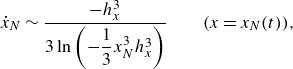
\begin{equation} \dot x_N \sim \frac { – h_x^3 }{ 3 \ln \left (- \frac {1}{3} x_N^3 h_x^3 \right ) } \qquad (x = x_N(t)), \end{equation}

giving the rate of change of the contact line in terms of the frontal interfacial slope of the quasi-static region

$h_x(x_N,t)$

. The frontal slope of the quasi-static parabolic solution (3.4) can be evaluated as

(3.12)

\begin{equation} h_x(x_N,t) = -\frac {2}{x_N}\left (\frac {3 t}{x_N} – \frac {H}{B}\right )\!. \end{equation}

Substituting (3.12) into (3.11), we obtain the ordinary differential equation

(3.13)

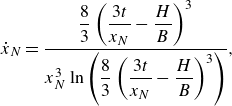
\begin{equation} \dot {x}_N = \dfrac {\dfrac {8}{3}\left (\dfrac {3 t}{x_N}-\dfrac {H}{B}\right )^3}{x_N^3\ln \left (\dfrac {8}{3}\left (\dfrac {3 t}{x_N}-\dfrac {H}{B}\right )^3\right )}, \end{equation}

yielding the desired explicit evolution equation for

$x_N(t)$

.

The ordinary differential equation (3.13) describes the contact-line evolution of the quasi-static regime, analogously to corresponding differential equations developed in the context of droplets, as considered in axisymmetric (Hocking Reference Hocking1982) and two-dimensional (King & Bowen Reference King and Bowen2001; Kiradjiev et al. Reference Kiradjiev, Breward and Griffiths2019) cases. A distinctive element in the present case is the pinning of one side of the parabolic interface by the injection nozzle, which introduces terms involving the parameter

$H/B$

, and results in an advancing centre of the parabola (as opposed to symmetrical spreading about a line source). We have thus drawn a link between the asymptotic structures that can underlie injection-driven pinch-off in capillaries and those encountered in the analysis of droplet spreading.

While (3.13) is the most reduced asymptotic form of the quasi-static ordinary differential equation (to be used in the asymptotic analysis of the next sub-section), for the numerical evaluation of the quasi-static theory, we opt here to integrate the unsimplified form (3.8) owing to the large

$\ln (\ln z)/\ln z$

residual in the expansion (3.10). We solve (3.8) with (3.12) numerically subject to an initial condition on

$x_N(t_0)$

using Runge–Kutta–Fehlberg integration. In order for the argument to be positive, as is required of the Lambert

$W$

-function here, we require the initial condition to satisfy

$x_N(t_0) \lt x_N^{(0)}\equiv 3Bt_0/H$

. As is common in intermediate asymptotics (Barenblatt Reference Barenblatt1996), the quasi-static states have an attractor to which the solutions converge that is independent of the initial condition (demonstrated here in Appendix B). Thus, to give space for the quasi-static attractor to establish, we initialise with

$x_N(t_0) = 0.8 \, x_N^{(0)}$

with

$t_0=5$

, and show the solution for

$t \geqslant 50$

, for which the solutions have closely approached the attractor.

With

$x_N(t)$

determined in this way, the parabolic profile (3.4) can be evaluated to give a prediction for the evolution of the interface, with pinch-off occurring critically once

$h_m(t_*) = 1/B$

, where

(3.14)

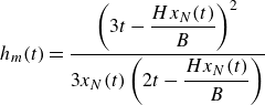
\begin{equation} h_m(t) = \frac {\left (3t-\dfrac {Hx_N(t)}{B}\right )^2}{3x_N(t) \left (2t-\dfrac {Hx_N(t)}{B} \right )} \end{equation}

is the maximum of the parabola. The prediction of the quasi-static theory is shown for

$H=0.05$

and

$H=0.4$

in figure 4. The left-hand panels show the quasi-static prediction for the (parabolic) interface profile as a red dashed line at the time of pinch-off, showing good agreement with the numerical prediction of the time-dependent necking-zone model. The evolution of the maximal thickness (3.14) is overlaid as a red, dashed line in the right-hand panels (

$d$

) and (

$f$

) of figure 4 (representing the relevant cases of small

$B$

), showing excellent agreement with the numerical predictions of the full necking-zone theory (2.23)–(2.25) over the required time scale,

$1 \ll t \leqslant t_*$

. The results confirm that the quasi-static regime is capturing the interface evolution for cases of

$B \ll 1$

.

3.2. Asymptotic solution to the quasi-static theory for

$H \ll 1$

For

$H \ll 1$

, the spacing between the nozzle and the sidewall is small relative to the size of the capillary. In this limit, the thickness of the film near the input nozzle can, similarly to the contact-line position (3.2), be approximated as zero on the scales of the outer quasi-static region for all times up to pinch-off

$(h(0,t) = H/B \ll 1/B)$

. As a result, the parabola is approximately symmetric (cf. figure 4

$e$

, where

$H = 0.05$

), with a line of symmetry residing close to

$x_N(t)/2$

. The solution thereby retains a self-similar interfacial shape, a simplification which affords a yet further reduced analytical prediction within the quasi-static theory.

The implication of

$H \ll 1$

within the quasi-static theory is that we can neglect the

$H$

term in the governing differential equation (3.11), which reduces it to the parameterless equation

(3.15)

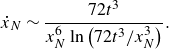
\begin{equation} \dot {x}_N \sim \frac {72t^3}{x_N^6\ln \left({72t^3}/{x_N^3}\right)}. \end{equation}

We now seek a leading-order asymptotic solution to (3.15) during the quasi-static time-scale (

$1 \ll t \leqslant t_*$

). To derive this, we try the ansatz of the form

(3.16)

\begin{equation} x _N( t ) \sim f( t ) t ^{\alpha } \qquad (t \gg 1), \end{equation}

where

$\alpha$

is an unknown constant to be determined and

$f( t )$

is an unknown function with the property that

$\ln (f( t )) \ll \ln t$

for

$ t \gg 1$

(in other words,

$f(t)$

is assumed to be at most of logarithmic order in

$ t$

or a power thereof). Substitution of (3.16) into (3.15) yields, on neglect of higher-order terms in

$t \gg 1$

,

(3.17)

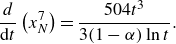
\begin{equation} \frac {{d} }{\textrm {d} t } \left( x _N^7 \right) = \frac {504 t ^3}{ 3(1- \alpha ) \ln t }. \end{equation}

Integrating, and using a change of variable in the integral

$z = 4 \ln t$

, we obtain

(3.18)

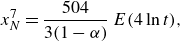
\begin{equation} x _N^7= \frac {504}{3(1- \alpha ) } \, E(4 \ln t ) , \end{equation}

where

$E(z) \equiv \int _\infty ^z z^{-1} e^{z} \; \textrm {d} z$

is the exponential integral function, and we have set the constant of integration to zero in order to satisfy the early-time asymptotic condition

$ x _N \to 0$

as

$ t \to 0$

. With use of the large-argument asymptote of the exponential integral function

$E(z) \sim e^z/z$

as

$z \to \infty$

(Abramowitz & Stegun Reference Abramowitz and Stegun1965), (3.18) reduces to

(3.19)

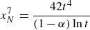
\begin{equation} x _N^7 \, = \frac {42 t ^4}{(1-\alpha )\ln t } \, \end{equation}

in the relevant limit

$ t \gg 1$

. Comparing the equation above with the ansatz (3.16), we see that

$\alpha = 4/7$

is necessary for consistency, and

$f( t ) = (98/\ln t )^{1/7}$

. Then, since

$\ln (f( t )) = O( \ln (\ln t ))$

, the derived function

$f(t)$

satisfies the required asymptotic property stipulated in our ansatz (3.16) that

$\ln (f( t )) \ll \ln t$

, confirming the asymptotic consistency of the derivation. We conclude that the position of the contact line evolves as

(3.20)

\begin{equation} x _N \sim \left ( \frac {98 t ^4 }{\ln t } \right )^{1/7} \qquad ( 1 \ll t \leqslant t_*). \end{equation}

The result of (3.20) indicates a dominant

$x_N \sim t^{4/7}/(\ln t)^{1/7}$

growth of the front of the necking disturbance for small

$B$

. The corresponding prediction of the maximum of the parabolic profile (3.4), occurring at

$ x = x _N( t )/2$

with (3.20), is

(3.21)

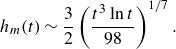
\begin{equation} h_m( t ) \sim \frac {3}{2} \left (\dfrac { t ^3 \ln t }{98} \right )^{1/7}. \end{equation}

The above is overlaid in figure 4(

$f$

) as blue crosses in the example with

$B=0.05$

and

$H=0.05$

, showing excellent agreement with both the numerical prediction of the full necking-zone theory (2.23)–(2.25), and the prediction of the quasi-static theory derived from solving the differential equation (3.8) numerically.

A

$t^{4/7}$

power component was likewise obtained for the contact-line position in the late-time regime of injection-driven spreading of a two-dimensional droplet along a precursor film, based on treating the logarithmic dependences that appear in (3.15) as constant (Kiradjiev et al. Reference Kiradjiev, Breward and Griffiths2019). Our analysis indicates that, in the context of the pinch-off problem, the additional slowly varying

$\ln t$

factor we derive in (3.20) is necessary for a consistent leading-order pinch-off solution that is sufficient to encompass the complete quasi-static time interval preceding pinch-off,

$1 \ll t \leqslant t_*(B)$

.

To determine the pinch-off time, we substitute (3.21) into the pinch-off criterion

$h_m( t _*) = 1/B$

, giving

(3.22)

\begin{equation} t _*^3 \ln \big( t _*^3\big)= a B^{-7}, \end{equation}

where

$ a = ({112}/{27} )^2$

is a numerical constant. Hence,

(3.23)

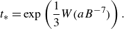
\begin{equation} t _* = \exp \left (\frac {1}{3}W\big( a {B^{-7}}\big)\right ) . \end{equation}

Since

$B \ll 1$

, we can simplify the above using (3.9) to give the final result

(3.24)

\begin{equation} t _* \sim \left ( \frac { a B^{-7}}{\ln \big( a B^{-7}\big) } \right )^{1/3}\sim 1.350 \left ( \frac {B^{-7}}{\ln (1/B) } \right )^{1/3}, \end{equation}

providing an explicit asymptotic prediction for the pinch-off time

$t_*$

for small capillary number. The prediction is overlaid as a dashed red curve in figure 5, showing agreement with the pinch-off time predicted by the numerical solution to the unsimplified necking-zone theory of (2.23)–(2.25) in the relevant limit of

$B \to 0$

. Despite being a theory based on

$H \ll 1$

(since, if

$H = O(1)$

, the parabolic interface is asymmetric during the dominant interval

$1 \ll t \leqslant t_*(B)$

and the contact line cannot conform to a simple asymptote of the form (3.16)), the prediction nonetheless appears to capture the

$B \to 0$

trend for cases of both

$H=0.05$

and

$0.4$

. The result of (3.24) implies that

$ t _* \gg 1$

as

$B \to 0$

and thus self-consistently predicts the existence of the large asymptotic time interval wherein the quasi-static regime occurs (

$1 \ll t \leqslant t_*(B)$

).

3.3. Conditions for consistency of the necking-zone model

The original theory of the necking zone (2.23)–(2.25) was based on two underlying asymptotic modelling assumptions: first, that lubrication theory applies to leading order in the necking zone; and second, that a long (Taylor) bubble forms. We now consider the parametric conditions under which these conditions hold self-consistently.

Beginning with the lubrication approximation (2.10), we note that, in our non-dimensional variables, the condition of small interfacial slopes can be expressed as

(3.25)

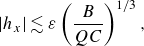
\begin{equation} |h_x| \lesssim \varepsilon \left ( \frac {B}{QC} \right )^{1/3}, \end{equation}

where

$\varepsilon \ll 1$

is a small dimensionless parameter characterising the size of the aspect ratio (representing the tolerance of the approximation), and

$Q=q_F/q_B$

is the ratio of the film flux to the bubble flux. Thus, the aspect ratio of the necking disturbance at the time of pinch-off can be characterised by

(3.26)

\begin{equation} h_x \sim \frac {h_m(t_*)}{x_N(t_*)} \sim 0.50 \, \left (B \ln \left (1/B \right ) \right )^{1/3}, \end{equation}

upon using

$h_m(t_*) = 1/B$

and

(3.27)

\begin{equation} x_N(t_*)\sim 2.0\,\left (\frac {1}{B^{4}\ln (1/B)}\right )^{1/3}, \end{equation}

obtained by substituting the pinch-off time (3.24) into (3.20). Equating (3.25) and (3.26), and simplifying, we obtain the constraint on

$Q$

and

$C$

given by

(3.28)

\begin{equation} QC \ln (1/C) \lesssim 12 \, \varepsilon ^3. \end{equation}

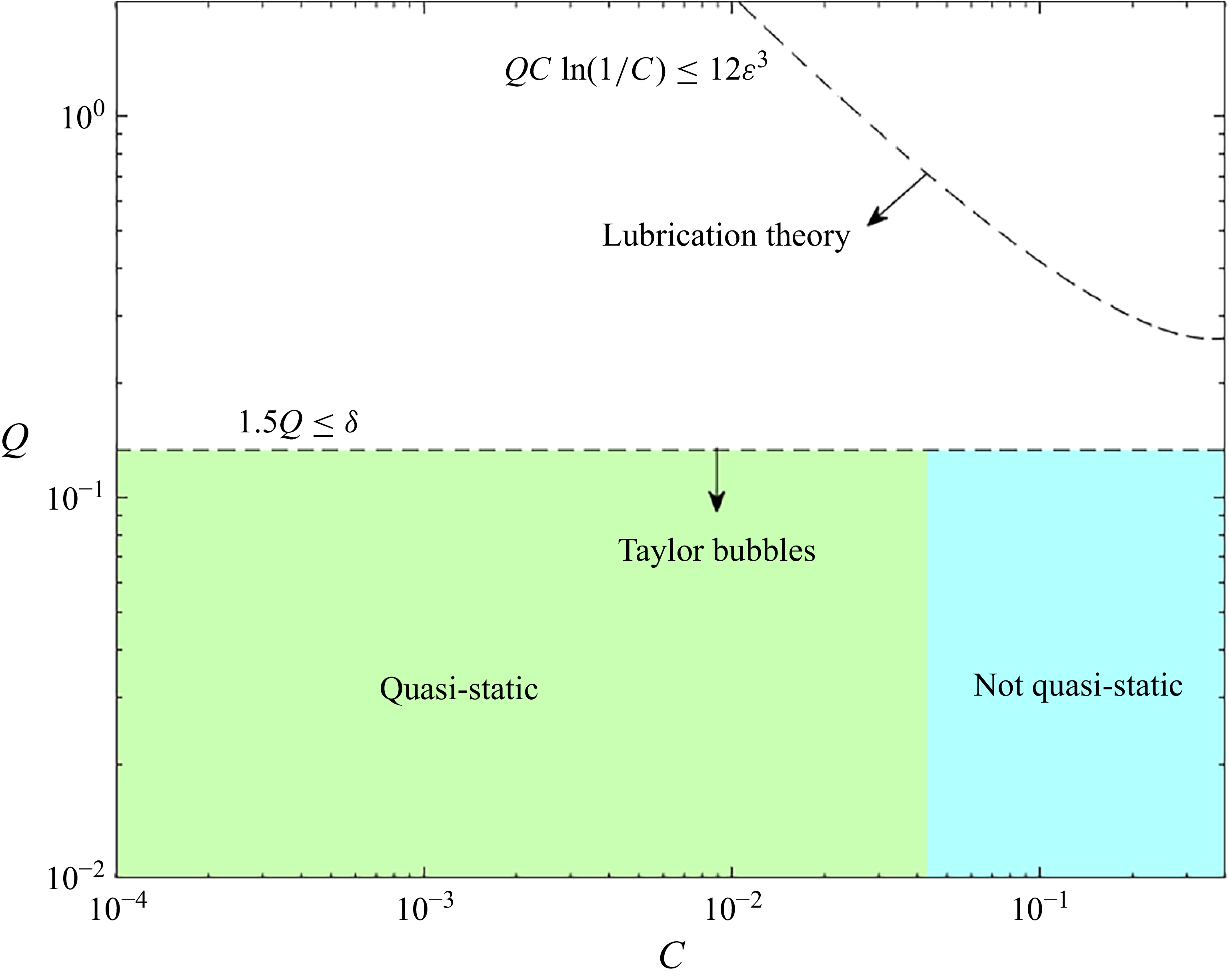
If the criterion above holds then the model prediction self-consistently maintains lubrication theory. The product

$QC \equiv \mu q_F / \gamma d$

can be interpreted as an alternative capillary number derived from the injection flux of the viscous phase (as opposed to the flux of the injected inviscid bubble phase used to define

$C$

). The result indicates that the film capillary number

$QC$

is the primary control in determining the self-consistency of lubrication theory. This finding is consistent with the fact that, similarly to a droplet driven by injection (e.g. Kiradjiev et al. Reference Kiradjiev, Breward and Griffiths2019), larger injection fluxes feeding the necking disturbance will cause it to thicken relatively faster than it spreads longitudinally, yielding steeper aspect ratios. There is a weak logarithmic dependence on

$C$

, stemming from its role in controlling the precursor-film thickness and, in turn, the spreading rate via the Cox–Voinov law. The constraint above restricts the region of validity of the model predictions in the parameter space

$(C,Q)$

below the locus plotted as a dashed curve in figure 6 for the illustrative value

$\varepsilon = 0.2$

. Lubrication theory is thus more strongly satisfied for smaller film capillary numbers

$QC \ll 1$

(verification that lubrication theory arises is confirmed by direct comparisons with full-Stokes simulations in Appendix C).

Figure 6.

The

$C$

–

$Q$

parameter space partitioned by the characteristic regions in which the two asymptotic assumptions of the model (3.28) and (3.30) hold self-consistently (coloured shading). The criteria, for illustrative tolerances of

$\varepsilon =\delta = 0.2$

, are shown as dashed curves, with the Taylor-bubble condition lying entirely inside the criterion for lubrication theory. Within the region of model self-consistency, the sub-region where quasi-static theory applies to good approximation is shown in green.

Second, we examine the self-consistency of the Taylor-bubble regime, defined by the property that the bubble cap extends characteristically further downstream than the scale of the necking disturbance (2.3), forming a long bubble,

(3.29)

\begin{equation} x_N(t_*) \ll x_F(t_*). \end{equation}

Using the dimensionless form of the prediction for the characteristic length of the Taylor bubble given below (2.9), namely

$x_F \sim Bt/Q$

, and (3.27), we find that, after some simplification, the ratio reduces to

(3.30)

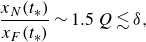
\begin{equation} \frac {x_N(t_*)}{x_F(t_*)} \sim 1.5\, Q \lesssim \delta , \end{equation}

where

$\delta \ll 1$

is a parameter representing the tolerance. Thus, it is indicated that the characteristic length of the bubble to the length of the necking disturbance is controlled independently by the flux ratio

$Q$

. For

$\delta = 0.2$

, the above yields

$Q \lesssim 0.1$

, indicating that well defined Taylor bubbles are formed if the flux of the viscous fluid is less than one tenth of the bubble flux. The condition is indicated by a horizontal dashed line on figure 6.

The region of

$(C,Q)$

space in which the Taylor bubble assumption (3.30) applies is entirely contained within the region where lubrication theory (3.28) applies. Since the self-consistency of the model requires both of these conditions to be satisfied, we conclude that, for tolerances of

$\varepsilon = \delta = 0.2$

, model self-consistency (represented by the coloured regions) occurs sufficiently on the basis of the Taylor-bubble condition alone. A decrease in tolerances moves the dashed lines representing validity of each condition closer together, with the conclusion that they remain separate holding for tolerances of

$\varepsilon \sim \delta \sim 0.1$

. For yet smaller tolerances, some overlap between the constraints of (3.28) and (3.30) is possible, with the lubrication constraint introducing some restriction on the flux ratio at moderate capillary numbers

$\gtrsim 10^{-1}$

. The subregion highlighted in green on the parameter space (figure 6) defines where the small-

$B$

asymptotic limit of the pinch-off time (3.24) is within 20 % of the pinch-off time predicted by the full unsimplified necking-zone model (2.23)–(2.25) for

$H=0.05$

. Thus, for characteristic values of

$C \lesssim 0.04$

, the analytical quasi-static theory (§ 3.1) begins to apply to good approximation.

4. Summary and discussion

Our analysis has developed a progression of models at three levels of asymptotic reduction. The first comprised the full model of the necking zone (§ 2.2) formed by coupling lubrication equations to nozzle conditions and a downstream condition connecting the interface to the interior thickness of the Taylor bubble (2.23)–(2.25). Solutions to this first model can be classified based on the dimensionless Taylor-bubble film thickness

$B$

and nozzle–wall spacing

$H$

. The second level, arising for small

$B \ll 1$

(equivalently, small capillary number,

$C \ll 1$

), forms a quasi-static theory defined by the outer region retaining an effectively instantaneously static meniscus, and evolves in response to a slow time scale associated with the advance of an effective dynamic contact line,

$x_N(t)$

, governed by a Cox–Voinov law. The regime is represented by the ordinary differential equation for the evolution of the contact line (3.13). The third level of simplification is the asymptotic solution (3.20) within the quasi-static theory that applies strictly in the limiting case where the nozzle is tightly fitting (

$H \ll 1$

). In this case, the self-similar propagation allows for a simple analytical form of the solution to the quasi-static theory over the time scales on which the quasi-static theory applies up to pinch-off. The result yields an analytical law for the time of pinch-off (3.24) that accurately captures the predictions of the original necking model in the relevant limit of small capillary number (equivalently,

$B \to 0$

; figure 5). Despite being derived on the basis of a tightly confining nozzle (

$H \ll 1$

), the result appears to capture the leading-order pinch-off time for

$ B \to 0$

and

$H = O(1)$

.

In order to see the parametric dependences of the predictions explicitly, we redimensionalise the results. Henceforth, variables will represent their dimensional versions, with non-dimensional variables indicated by hats. The general predictions of the full necking-zone theory (§ 2.2) can be expressed as

(4.1)

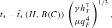
\begin{equation} t_* = \hat {t} _*\left (H, B(C) \right ) { } \left ( \frac {\gamma h_T^7} {\mu q_F^4}\right )^{1/3}, \end{equation}

where

$B(C)$

is the parameterless dimensionless function of the bubble capillary number

$C\equiv \mu q_B / \gamma d$

reviewed in figure 2,

$h_T = B(C) d$

is the interior thickness of the Taylor bubble given generally by (2.6) and

$\hat {t} _*(H,B)$

is the numerically determined dimensionless solution for pinch-off times shown in figure 5. Since neither

$H$

nor

$B(C)$

depend on the flux of the viscous fluid

$q_F$

, we note that the dependence of the pinch-off time on the simple inverse

$4/3$

power law of the viscous fluid flux

$q_F$

in (4.1) is a universal scaling.

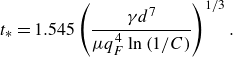
For capillary numbers

$C \lesssim 0.01$

, we derived an explicit theoretical prediction for the pinch-off time (3.24), which takes the dimensional form

(4.2)

\begin{equation} t_* = 1.545 \left (\frac {\gamma d^7}{\mu q_F^4\ln \left ( 1/C\right ) }\right )^{1/3}. \end{equation}

The result predicts that the time to bubble pinch-off is controlled by an inverse proportionality to the

$4/3$

power of the input flux of the viscous fluid

$q_F$

, a

$1/3$

power of the ratio of the surface tension to the fluid viscosity

$\gamma /\mu$

, and a

$7/3$

power of the channel half-width

$d$

. The prediction includes a weak logarithmic dependence of the pinch-off time on the bubble flux

$q_B$

contained in the capillary number

$C\equiv \mu q_B / \gamma d$

.

To provide an order-of-magnitude indication of the time scale (4.2), one can substitute representative microfluidic values. For an illustrative air–water microfluidic system (

$\mu = 10^{-3}\, \mathrm{Pa}\, \mathrm{s}$

and

$\gamma = 0.072\, \mathrm{N}\, \mathrm{m}^{-1}$

) with illustrative capillary width

$d=100\,\mu \mathrm{m}$

, capillary number

$C\sim 10^{-3}$

and film fluxes per unit width

$q_F$

in the range

$0.1$

–

$1\,\mu \mathrm{m^2\,s^{-1}}$

, one obtains characteristic pinch-off times of order

$t_* \sim 0.1{-}1\,\mathrm{ms}$

. Such an estimate is necessarily indicative, since the representative microfluidic parameters are drawn from experimentally realised microfluidic configurations (e.g. Garstecki et al. Reference Garstecki, Gañán-Calvo and Whitesides2005a
, Reference Garstecki, Fuerstman, Stone and Whitesides2006; Fu et al. Reference Fu, Ma, Funfschilling and Li2009; Deng & Schroën Reference Deng and Schroën2024) that differ in geometry from the idealised planar channel considered in the present paper. Hence, the comparison is intended only at a level of physical scale rather than quantitative agreement.

Finally, we note that the maximal size of the necking disturbance, as represented by

$x_N(t_*)$

and non-dimensionally by the prediction of (3.27), is

(4.3)

\begin{equation} x_N(t_*) \sim 2.3 \, \left (\frac {\gamma d^4 }{\mu q_F\ln (1/C)}\right )^{1/3}. \end{equation}

The result shows that the maximal length of the necking disturbance is controlled by a

$4/3$

power of the channel size

$d$

, a

$1/3$

power of the ratio of the surface tension to the fluid viscosity

$\gamma /\mu$

and an inverse proportionality to the

$1/3$

power of the input flux of the viscous ambient phase

$q_F$

. Thus, the length of the necking zone is primarily controlled by the width of the channel. Similarly to (4.2), there is a very weak logarithmic dependence of the maximal length of the necking zone on the bubble flux

$q_B$

contained in the capillary number

$C$

.

4.1. Theory limitations

The theory provided in this paper describes an asymptotically self-consistent lubrication regime. As shown by the parametric conditions for asymptotic consistency (§ 3.3), the analysis here is limited to predict the time up to pinch-off of a long (i.e. Taylor) and inviscid bubble. First, we note that lubrication theory breaks down immediately after pinch-off, owing to the development of infinitely steep interfaces on either side of the pinch-off point. The newly detached interfaces at both the rear of the newly formed bubble, and at the nose of the remnant of bubble fluid attached to the input nozzle, will both exhibit infinitely steep gradients. Hence, solutions (like the one shown in figure 3) are valid up to the point of pinch-off, but lubrication theory cannot necessarily capture the dynamics immediately after pinch-off. Full (nonlinear) curvature and full-Stokes flow may be required to resolve the newly formed cap and bubble rear. Moreover, if we were to consider larger flux ratios for which short or approximately circular-cross-sectioned bubbles are generated at flux ratios of order unity (situations above the horizontal dashed line shown in figure 6), similar full-Stokes considerations may be required. In this case, the flow would no longer form a Taylor bubble to which we can match the necking zone via a precursor-film condition of the form (2.19). The necking dynamics would instead interact more directly with the developing bubble, likely necessitating both nonlinear curvature and full-Stokes resolution.

We acknowledge that the analysis presented in this work is restricted to the planar coflow geometry. Extension of this analysis to the axisymmetric geometry would be of interest, and the demonstration of the quasi-static regime in the two-dimensional case presented here provides a first step towards this. In the axisymmetric case, the analogue of the parabolic quasi-static states would be surfaces of minimum curvature connecting two concentric annuli. Analysis of similar states in the static context, described by the axial Young–Laplace equations (e.g. Slobozhanin, Alexander & Fedoseyev Reference Slobozhanin, Alexander and Fedoseyev1999; De Gennes, Brochard-Wyart & Quéré Reference De Gennes, Brochard-Wyart and Quéré2003; Collicott, Lindsley & Frazer Reference Collicott, Lindsley and Frazer2006; Lv & Hardt Reference Lv and Hardt2021), shows that the static states exhibit a rich variety of forms (relative to the universally parabolic states arising here), as well as the possibility for minimising surfaces not to exist, or to bifurcate.

Finally, we note that the underlying asymptotic structure of the quasi-static theory assumes an inviscid bubble, as is typical in classical studies of Taylor bubbles (e.g. Fairbrother & Stubbs Reference Fairbrother and Stubbs1935; Bretherton Reference Bretherton1961). If the bubble viscosity is appreciable, a zero pressure gradient no longer applies in regions where the interface is flat, and hence the parallel flow solution is no longer applicable. Consequently, the asymptotic structure of a Taylor bubble, containing a broad interior region with a near-uniform film thickness, no longer exists. An interesting theoretical question would be to explore the implications of finite bubble viscosity.

4.2. Comparisons

The generation of Taylor bubbles has received significant experimental attention (e.g. Cubaud et al. Reference Cubaud, Tatineni, Zhong and Ho2005; Xiong et al. Reference Xiong, Bai and Chung2007; Fu et al. Reference Fu, Funfschilling, Ma and Li2010; Lu et al. Reference Lu, Fu, Zhu, Ma and Li2016; Li, Wu & Chen Reference Li, Wu and Chen2021; Huang & Yao Reference Huang and Yao2022). Many experimental investigations have aimed to correlate bubble characteristics (such as pinch-off time or, equivalently, bubble length or volume) and dimensionless parameters of the system, such as capillary number. Cubaud et al. (Reference Cubaud, Tatineni, Zhong and Ho2005) determined a linear relationship between the length of a bubble formed in a cross-flow junction of square cross-section, and the inverse of the liquid volumetric flux fraction. The scaling is also validated in the coflow geometry by Xiong et al. (Reference Xiong, Bai and Chung2007), who use an experimental particle image velocimetry system to provide a visual depiction of the interface with time, with the interface appearing approximately parabolic near to the nozzle (figure 7d of Xiong et al. Reference Xiong, Bai and Chung2007), exhibiting qualitative agreement with the predictions of the necking-zone theory in § 2.2.

Although there are no identical experimental or numerical studies on Taylor bubble formation in a planar coflow geometry, we can draw qualitative comparisons with existing empirical scaling laws. Assuming the Taylor bubble takes an approximately cylindrical shape, the scaling law proposed by Cubaud et al. (Reference Cubaud, Tatineni, Zhong and Ho2005) is analogous to a prediction of pinch-off time given by

$t_* \propto 1/q_F$

. This inverse scaling for pinch-off time is also evidenced by the experimental investigation of Salman et al. (Reference Salman, Gavriilidis and Angeli2006) into the formation of Taylor bubbles by coaxial injection of air into a small cylindrical channel filled with water. The progression of the air–water interface is recorded with a high-speed camera and, from photographic observations, the frequency of bubble production is concluded to increase with the flux of either fluid phase. They also conclude that the period of bubble formation exhibits only a weak dependence on the surface tension of the outer liquid, and is determined predominantly by the nozzle size and flow rates. The prediction for pinch-off time of Taylor bubbles as

$t_* \sim q_F^{-1}$

, derived implicitly from the scaling law for bubble length given by Cubaud et al. (Reference Cubaud, Tatineni, Zhong and Ho2005), is qualitatively consistent with the findings of the present paper that

$t_* \sim q_F^{-4/3}$

, and we speculate that the different power is due to the differing geometries. As noted above in § 4.1, our analysis could be extended to address the more complex geometries associated with a cylindrical capillary or microchannel of square cross-section, which could in principle be addressed by appropriately adapting or generalising the necking theory and quasi-static frameworks. Similarly, we anticipate some of the ideas presented herein could potentially be applied to other related bubble systems including Hele-Shaw cells (e.g. Hazel & Heil Reference Hazel and Heil2002; Gaillard et al. Reference Gaillard, Keeler, Le Lay, Lemoult, Thompson, Hazel and Juel2021; Lawless et al. Reference Lawless, Keeler, Hazel and Juel2024).

5. Conclusions

This paper has presented three primary developments. First, we determined a new theory for the necking dynamics of an intruding Taylor bubble, based on lubrication theory with matching to the Taylor bubble thickness downstream. Second, we introduced principles of quasi-static modelling and contact-line matching to the problem of capillary pinch-off, revealing a link between droplet dynamics and pinch-off dynamics. Third, we used this framework to develop an analytical prediction for pinch-off time of an injected bubble, applicable in the limit of small capillary numbers where the asymptotic structure becomes most refined

(5.1)

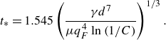
\begin{equation} t_* = 1.545 \left (\frac {\gamma d^7}{\mu q_F^4\ln \left ( 1/C\right ) }\right )^{1/3}. \end{equation}

The result represents the first analytical theory for injection-driven pinch-off in a capillary system derived from first principles. The result holds in the case of a classical inviscid Taylor bubble for which the region downstream of the necking disturbance becomes uniform and stagnant to leading order. As viscous fluid is introduced, the viscous film bulges with a shape controlled by surface tension maintaining a minimising (quasi-static) surface. The analysis highlights that the swelling of this surface is moderated by advancement of a frontal effective contact line; that is, the visco-capillary dynamics at the front of a quasi-static necking disturbance control the dimensions of the necking bulge. Our analysis thus elucidates a new interpretation for how bubble pinch-off is controlled crucially by a minimising surface that evolves in response to its coupling with a frontal contact line.

The result shows that the time to bubble pinch-off in this planar geometry exhibits a

$q_F^{-4/3}$

power-law dependence on the flux of the liquid phase, but is almost independent of the flux of the bubble phase, with only a logarithmic dependence contained within the capillary number

$C$

(stemming from its control of the interior Taylor-bubble thickness to which the necking zone is matched). The prediction also reveals a large

$d^{7/3}$

power-law dependence on the half-width of the geometry, and a

$(\gamma /\mu )^{1/3}$

power dependence on the ratio of the surface tension coefficient to the liquid viscosity.

The analysis of this paper has focused on the two-dimensional flow of a Newtonian, inviscid bubble within a straight-walled channel of uniform width. The framework presented here provides a basis for various potential generalisations of the quasi-static analysis to more complicated injection geometries (such as cylindrical capillaries, cross-flow or flow-focusing configurations), to Hele-Shaw systems and to configurations where the inviscid bubble is replaced with a fluid of non-negligible viscosity or a non-Newtonian fluid, for example. Each of these presents an interesting direction for future development, for which the analysis of the present paper provides a foundation.