
We begin by introducing the multistate modeling framework in the context of chronic disease research, which serves to highlight the key challenges and distinctive features of applying such models in this domain. We then extend the framework to accommodate transitions across latent multimorbidity patterns, which represent clusters of co-occurring diseases. Figure 1 presents an overview of the proposed methodology and conceptual framework, offering a graphical summary of our approach.
Multistate modeling framework
A multistate model describes a stochastic process, \(S(t), \, t > 0\), that records subjects’ moving across a set of discrete health states, \(\mathscr {S}\)15,16, over time. \(\mathscr {S}\) contains a number of transient states, reflecting different health-living states, and “Death” as the absorbing state, i.e. subjects cannot exit this state and transition to others. Time is treated as a continuous variable, allowing transitions between states to occur at any moment—a realistic assumption when modeling medical and biological processes. Specifically, the timescale used in the multistate models considered here is the individual’s age. Consequently, each subject may have a different time origin in the model, corresponding to their age at study entry.
In the context of aging and the development of chronic conditions, it is highly unlikely that transitions between health states are recorded at the exact moment they occur. Only acute health events typically allow for precise timing of state changes. More commonly, individuals are assessed at discrete intervals–such as during routine medical visits or scheduled health surveys–and transitions are inferred from these periodic observations. This observation mechanism results in panel data, characterized by intermittent observation and interval censoring: while it is known that a transition occurred between two observation points, the exact timing remains unknown. In addition, unlike continuous monitoring, which captures every state transition in real time, panel data provide only snapshots of an individual’s health status at specific time points. As a result, the complete sequence of states occupied during the observation period is often partially observed, and some transitions may go undetected. Traditional multistate models, however, assume continuous observation and precise tracking of state changes, which may not align with the realities of such data.
To address this, our work employs multistate modeling approaches specifically designed for panel data, which account for the intermittent nature of observations during parameter estimation. Importantly, we assume that observation times are non-informative—that is, the timing of measurements is independent of the underlying multistate process. Additionally, we adopt the Markov assumption, meaning that the probability of transitioning to a future state, and the timing of that transition depend solely on the current state and the individual’s current age:
$$\begin{aligned} \Pr [S(t+h) = y \mid S(r) = s(r), \, r \le t] = \Pr [S(t+h) = y \mid S(t) = S(t)], \quad \forall h > 0. \end{aligned}$$
(1)
A multistate model is uniquely defined by a set of transition intensity functions, \(q_{ij}(t, x)\), which represent the instantaneous probability at each time t of moving between each pair of states \(i\) and \(j\), for \(i\), \(j\) \(\in \mathscr {S}\). In the continuous-time case, the transition intensities can be represented in a \(nxn\) matrix \(Q\), with \(n\) total number of states, whose rows sum to zero. The Kolmogorov Forward Equations (Chapman–Kolmogorov Differential Equations) are used to describe the evolution of probabilities over time in a Continuous Time Multistate Models (CTMM). These equations provide a mathematical framework to calculate the probability of being in a specific state at any given time. Let \(P(t)\) represent the \(n \times n\) matrix of state probabilities, where \(p_{ij}(t)\) is the probability of being in state \(j\) at time \(t\), given that the process started in state \(i\) at time 0. The Kolmogorov Forward Equation is given by:
$$\begin{aligned} \frac{dP(t)}{dt} = P(t) \cdot Q \end{aligned}$$
(2)
For each state pair \((i, j)\), the derivative \(\frac{dp_{ij}(t)}{dt}\) represents the instantaneous rate of change of the probability of being in state \(j\) at time \(t\), starting from state \(i\). In the context of aging and chronic diseases, the matrix, \(Q(t)\), of the transition intensities needs to be allowed to vary with time, allowing the probability of transitions across the state to vary as the individual ages. As a result, the solution of the Kolmogorov Forward Equations (KFEs) becomes more complex as it requires integration over time. Direct integration requires the use of numerical solvers17, which can be more computationally intensive and time-consuming. Alternatively, a numerical approximation that uses a piecewise constant version of the \(Q(t)\) matrix can be used to simplify computations. To approximate the solution in the time-inhomogeneous case, the time interval \([0, t]\) can be divided into small subintervals \([t_i, t_{i+1}]\), where \(\Delta t = t_{i+1} – t_i\) is the step size. The transition intensity matrix \(Q(t)\) is approximated as piecewise constant within each interval. This leads to the following approximation of the solution:
$$\begin{aligned} P(t) \approx P(t_0) \cdot \prod _{i=0}^{n-1} e^{\Delta t \cdot Q(t_i)} \end{aligned}$$
(3)
A crucial step in the modeling process involves selecting a parametric form for the intensity function. We adopt the proportional hazards model due to its interpretability and widespread use in clinical research. While alternative parametric families could theoretically be considered, this study focuses on the Gompertz distribution, which reflects the natural tendency of transition intensities—such as progression to greater disease burden or death—to change monotonically with age. This choice aligns with well-documented patterns in health and disease progression18,19,20. According to this parametric proportional-hazard model, covariates \({\textbf {x}}\) associated with transition intensities are assumed to have a multiplicative effect, and each transition \(i \rightarrow j\) can have a different set of covariate effects. The transition intensities take the form:
$$\begin{aligned} h_{ij}(t | x) = \lambda _{ij} e^{\alpha _{ij} t + \beta _{ij}^T {\textbf {x}}} \end{aligned}$$
(4)
where \(\lambda _{ij}\) is the baseline rate parameter in exponential form for the transition from state \(i\) to \(j\), \(\alpha _{ij}\) the shape parameter for the transition from state \(i\) to \(j\), \({\textbf {x}}\) the vector of covariates and \(\mathbf {\beta _{ij}}\) the vector of regression coefficients. When \(\alpha <0\), the hazard decreases over time, whereas \(\alpha >0\) characterizes an increasing hazard with age. For \(\alpha =0\), the Gompertz model reduces to the exponential model, i.e. a time-homogeneous model.
Hidden multistate models for latent multimorbidity patterns
Multimorbidity states are conceptualized as latent constructs—unobservable directly but inferred from a set of categorical disease indicators, denoted as \({\textbf {Y}}(t) = (Y_1(t), Y_2(t), \dots , Y_R(t))\), where each \(Y_r(t)\) indicates the presence or absence of a specific chronic condition at age t. The probability that an individual k belongs to a particular multimorbidity pattern, conditional on the diseases developed by time t, is given by \(P(C_k(t) = c \mid {\textbf {Y}})\), where \(c \in \{1, 2, \dots , C\}\). This probability can be estimated using existing unsupervised learning techniques, such as Latent Class Analysis (LCA) or other soft-clustering methods. Let \(\hat{P}(C_k (t) = i \mid {\textbf {Y}})\) denote the posterior probability that the individual \(k\) belongs to the latent class \(i\) estimated from the latent class model.
Based on the observed values \({\textbf {y}}(t)\), an individual can be assigned to the most likely pattern using this probability, resulting in the observed state W(t). However, when analyzing transitions between latent multimorbidity states, it is important to recognize that only W(t) is observed, not the true latent state C(t). This problem can be framed as a hidden multistate model that extends the classical framework by explicitly modeling the generation of the observed states from the latent (hidden) ones21. For each individual k, at observation time \(t_{kn}\), the observed states W are generated conditionally on the latent states C via an emission matrix E. This is an \(n \times n\) matrix, where the entry (i, j) represents the probability of observing state j given that the hidden state is i. The emission probabilities are defined as:
$$\begin{aligned} e_{i,j} = P(W(t) = j \mid C(t) = i) \end{aligned}$$
(5)
In practice, these probabilities are estimated using posterior class-membership probabilities obtained from the latent class model, as defined above. Then, the emission probabilities can be estimated as22:
$$\hat{e}_{i,j} = \frac{\sum _{k=1}^N \textbf{1}(W_k = j)\, \hat{P}(C_k = i \mid Y_k)}{\sum _{k=1}^N \hat{P}(C_k = i \mid Y_k)}.$$
where N is the total number of individuals in the sample. This estimator approximates the joint distribution \(P(W, C)\) using posterior expectations and normalizes to obtain \(P(W \mid C)\). The emission matrix is assumed to be time-invariant, as it depends only on the measurement model derived from the baseline latent class analysis.
Since exact states are unknown, subject k’s contribution to the likelihood23 needs to be calculated over all possible paths of underlying states \(C_{k1}, \ldots , C_{k n_k}\):
$$\begin{aligned} L_k = \Pr (w_{k1}, \ldots , w_{k n_k}) = \Pr (w_{k1}, \ldots , w_{k n_k} \mid C_{k1}, \ldots , C_{k n_k}) \Pr (C_{k1}, \ldots , C_{k n_k}) \end{aligned}$$
(6)
Assuming that the observed states are conditionally independent given the values of the underlying states and the Markov property, the contribution \(L_k\) can be decomposed into sums over each underlying state. The sum is accumulated over the unknown first state, the unknown second state, and so on until the unknown final state:
$$\begin{aligned}&L_k = \sum _{C_{k1}} \ldots \sum _{C_{k n_k}} \Pr (W_{k1} \mid C_{k1}) \Pr (C_{k1}) \cdot \Pr (W_{k2} \mid C_{k2}) \Pr (C_{k2} \mid C_{k1}) \cdots \Pr (W_{k n_k} \mid C_{k n_k}) \nonumber \\&\Pr (C_{k n_k} \mid C_{k n_k-1}), \end{aligned}$$
(7)
where \(\Pr (W_{kn} \mid C_{kn})\) is the emission probability from the hidden state \(C_{kn}\) to the observed state \(W_{kn}\). The emission probabilities are treated as fixed quantities, estimated in the preliminary step as explained above, and then incorporated into the likelihood. The term \(\Pr (C_{k,j+1} \mid C_{kj})\) is the \((C_{kj}, C_{k,j+1})\)-th entry of the Markov chain transition probability matrix \(P(t)\), evaluated at \(t = t_{k,j+1} – t_{kj}\). If the hidden state is death, measured without error, whose entry time is known exactly, then the contribution to the likelihood is summed over the unknown state at the previous instant before death.
Fig. 1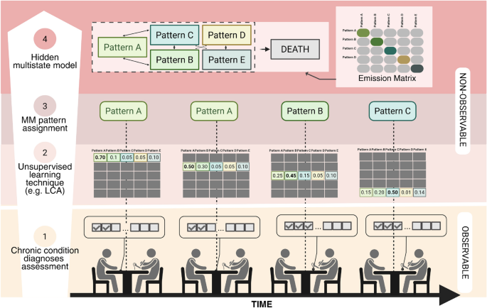
Conceptual and analytical pipeline for modeling multimorbidity trajectories. Chronic disease diagnoses are first aggregated using Latent Class Analysis to identify multimorbidity patterns (Steps 1–2). Individuals are assigned pattern membership at each visit (Step 3), and transitions across latent states—including progression to death—are modeled using a continuous—time hidden multistate model that accounts for misclassification and interval censoring (Step 4). LCA: Latent Class Analysis; MM: Multimorbidity. Created in BioRender.