

Annotation phaseInter-operator correspondence
Ground-truth labelling was assessed via one-to-one IoU matching at a 0.50 threshold and summarized by F1-0.50. The double-annotation yielded F1-0.50 ≈ 0.92, with 92% agreement on frame-level defect presence. All subsequent analyses employ the adjudicated consensus labels, and this correspondence level did not alter the comparative ranking of inspection modes.
Ground – truth labelling
Although the annotation phase of the dataset is a fundamental part of the development of a deep learning (DL) inspection tool, it is generally not included in the results discussion.
However, this work aims at comparing different inspection strategies that involve both data acquisition and data inference. Data collected for training the detection algorithms differ based on the chosen inspection mode, inevitably affecting the annotation phase. For each inspection mode, the number of annotated defects per image was counted for all retrieved frames related to the same sample. Since the total number of frames might change for each sample due to slight differences in raw video length, the average number of defects per image (avg_ngt) was calculated. Figure 5 shows the average number of defects per image for each sample under different inspection modes.
Fig. 5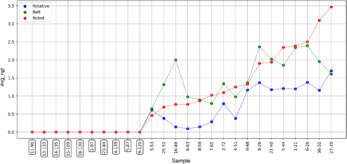
Average number of labelled defects per sample for different images acquisition techniques.
Each sample is assigned two numbers: the first number corresponds to its numbering within a specific category (defective, mildly defective, or normal), while the second number represents its absolute numbering across all samples. This dual numbering system helps distinguish between the sample’s position within its category and its overall position in the dataset. The framed labels on the x-axis correspond to the normal samples, while the others relate to defective samples. The data are arranged according to the increasing average number of annotated defects for Mode I. Considering only the defective samples, an increasing trend in the average number of annotations per image is observed for all three inspection modes. Despite the weld-lines always appearing in the same position and number due to the systematic behavior of the injection molding (IM) process, the extent of the defects can vary significantly from sample to sample. Moreover, the visibility of defects significantly depends on the inspection mode, with Mode I showing the lowest avg_ngt, while Mode II and Mode III show comparable results. Moreover, within the same inspection mode, different light reflections may either enhance the defect or cause it to nearly disappear. This inevitably affects the ability of the inspector to spot them while annotating the dataset. An example is reported in Fig. 6, which shows different frames of a defective sample for each inspection mode. Despite the images belonging to the same inspection video, it is clearly noticeable that some perspectives enhance defect visibility, while others make it almost impossible to detect. From a practical point of view, different images of the same part will thus be labeled either as defective or normal when annotating the dataset.
Fig. 6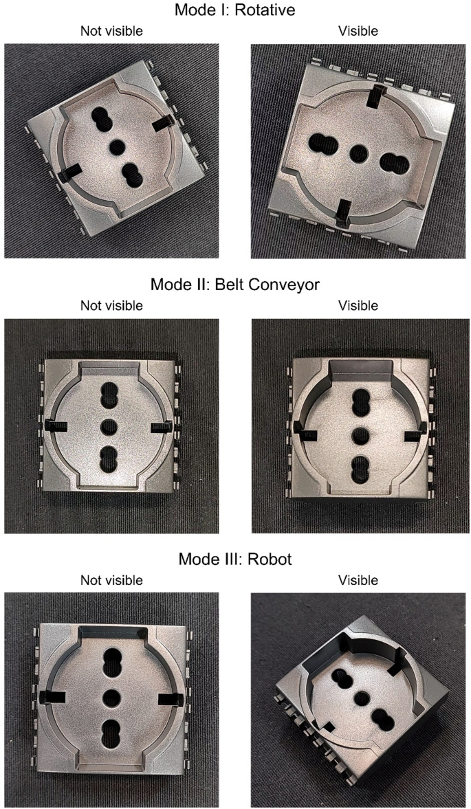
Comparison of defect visibility for different inspection modes for a reference sample (Part 1–21).
Detection performance
For the detection results, the inference time of the algorithm was first considered. For YOLO-v8s, using 1024 × 1024 p images, the inference time was around 70 ms, making the detection algorithm suitable for this manufacturing context. Frames from the videos of the testing samples were sampled with a time interval of 2 s, resulting in 50 frames per sample.
The inference results on the testing dataset are shown in Fig. 7.
Fig. 7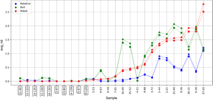
Average number of detected defects per sample for different inspection techniques. Round-shaped markers: nd, square-shaped markers: ndt.
The data are arranged as before, according to the increasing average number of detected defects (avg_nd) for Mode I. Both the average number of defects per sample across all inspected frames (avg_nd), and the average number of correctly detected defects per sample (avg_ndt) are reported. While avg_ndt is useful for providing insights about the precision of the inspection method, avg_nd allows for an immediate understanding of potential erroneous detections when considering the good samples, as avg_nd can assume values greater than zero even though no defects were labeled in the analyzed image. Considering avg_ndt, it is observed that Mode I exhibits a significantly lower average number of detected defects across all samples compared to Mode II and Mode III. This suggests that rotating the part around its axis is not effective in enhancing the visibility of the weld-lines. The performance of Mode II and Mode III are almost the same, with some outliers in Mode II data due to the belt conveyor inspection strategy. In this strategy, the part is observed from a stationary camera during transportation, and only the angle φ between the camera axis and the part’s position on the belt changes. Therefore, initial positioning can significantly affect the inspection results. Another important observation is the presence of avg_nd values different from zero for some normal samples, indicating false positives. Figure 8 shows the average false positive rate per sample (avg_fp_rate). A non-zero fp_rate means the algorithm detects defects not matched by any ground truth annotations, leading to the rejection of good parts. Despite similar fp_rate values across all three modes, Mode II performs the worst in terms of false positives, with several normal samples erroneously classified as defective. In contrast, Mode III shows better robustness against false positives, as it only misclassifies defective parts.
For the localization accuracy of the detected defects, the Intersection over Union metric (IoU) was considered. However, in our dataset the manually drawn bounding boxes are intended to simply enclose the defect region and their exact extent is inherently annotator-dependent (the same defect can be boxed slightly larger or smaller without affecting the inspection outcome). Therefore, very high IoU values are neither strictly expected nor required for the application, and IoU is treated here as a secondary indicator of localization consistency rather than a primary performance target. As shown in Fig. 9, the IoU ranges from 0.38 to 0.42 for almost all the samples. The IoU values indicate moderate localization consistency, which is acceptable for the present application because the inspection outcome depends primarily on detecting the presence of the weld-line defect rather than on highly accurate bounding-box localization. No significant differences can be observed between different modes, as the IoU is rather a characteristic of the detection algorithm itself, despite slightly lower results obtained with Mode I, which can be attributed to less accurate annotations. It is worth noting that for the inspection mode Mode I (Rotative), some data are missing (Sample 6–63, 7–65, 8–59, 16–49). This is due to the fact that for those samples, no defects were detected within these samples using this inspection method, thus no value of the IoU metric could be calculated. This is also confirmed by looking at Fig. 5, where, even though avg_nd ≠ 0, the value of avg_ndt = 0 for the above-mentioned samples.
The most crucial aspect of an AOI system is not missing any defective parts. In Mode II, some defective samples have both avg_nd and avg_ndt close to zero, indicating false negatives. These samples had defects that were only slightly visible but sufficient for the inspector to classify them as defective during annotation. Mode III, however, was able to recognize these defects in at least some frames, highlighting its effectiveness due to a wider range of inspection angles.
Fig. 8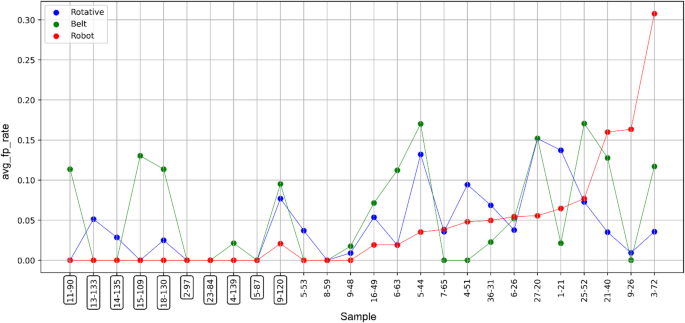
Average false positive rate per sample for different inspection techniques.
Fig. 9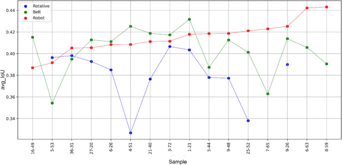
Average Intersection-over-Union for the defective samples. Missing data means that no defects were detected with that specific technique.
It is common practice to evaluate algorithm performance using the false negative rate (fn_rate) on the testing set. However, this approach may lead to erroneous conclusions. Figure 10, for example, might suggest similar detection capabilities for Mode II and Mode III. However, these results refer to specific frames, not sample. Despite comparable avg_fn_rate values, Mode III’s robot-based inspection strategy proved capable of detecting defects even in challenging scenarios where defects were only slightly visible.
Another crucial factor in quality control is the number of inspections per part. While it is a shared opinion that more inspections lead to more effective control, this aspect is often not deeply discussed. The maximum number of inspections depends on the production rate and the algorithm’s inference speed. In the IM process, cycle time can increase significantly with the part’s thickness due to longer cooling times, allowing for deeper inspection. In such cases, using an inspection video with varying observation angles can thus be more effective than static images. The available time and the algorithm’s inference speed determine the choice between static images and videos. Figure 11 shows the average number of detected defects (avg_nd) for different samples, varying the percentage of total frames used for inspection.
Fig. 10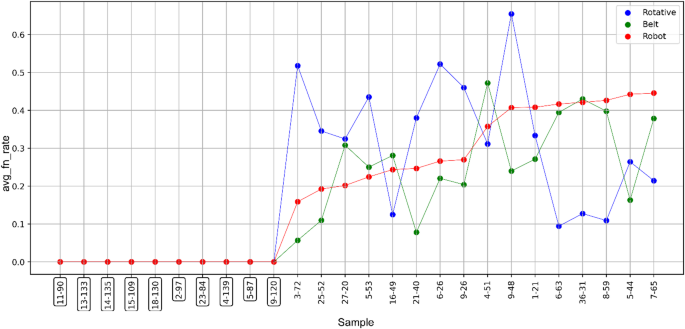
Average false negative rate per sample for different inspection techniques.
Fig. 11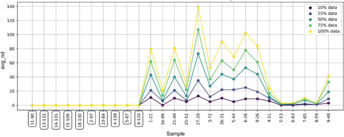
Average number of detected defects per sample for different percentages of frames used during the inspection.
The increasing number of frames can be interpreted as a transition from static images to videos. As the number of inspection frames per sample increases, the number of detected defects rises almost linearly. Having multiple detection results also allows for a decision-making strategy to reject or accept the part based on a defect detection threshold rather than the results of a single frame.
The choice of the aggregation threshold K is context-specific and depends on the inspection protocol, in particular on the number of frames evaluated per part and on defect observability across views. The part-level good/defective decision is based only on predicted detections aggregated over the inspected frames, while matched detections are used only offline for performance evaluation against the annotated ground truth.
In a real production environment, the final part-level decision can only rely on the inference output of the detector, since ground-truth information is not available during inspection. Therefore, the good/defective classification must be based on predicted detections aggregated over the inspected frames, while matched detections are used only offline to evaluate the system performance against the annotated ground truth. No universal aggregation threshold can be defined, as the decision rule depends on the specific application and on the acceptable trade-off between false positives and false negatives. In many industrial contexts, rejecting a good part is preferable to allowing a defective part to pass inspection; therefore, even a single predicted detection may be used to trigger a warning or a conservative rejection decision. In this work, K was fixed a priori to K = 3 and held constant across setups to ensure a consistent part-level decision policy. A possible direction for future work is to consider a continuous notion of defect “visibility” across the inspected sequence, instead of fixed-threshold policies, to better adapt the decision rule to varying defect entity.
After completing the inspection of each sample, it is possible to determine whether the part should be classified as defective or normal. The analysis of the metrics discussed reveals that, while these evaluation metrics guide the decision to accept or reject a part, there is still room for additional considerations. For instance, even though the detection algorithm may identify defects in a specific frame, setting a minimum number of correctly identified defects for each complete inspection can help address the issue of false positives. Conversely, developing a strategy that focuses on increasing recall can significantly reduce the risk of failing to detect defective parts. In most manufacturing scenarios, it is generally more critical to prevent an anomaly from going undetected than to avoid rejecting a good part. However, this priority can vary depending on the specific circumstances (Fig. 12).
Fig. 12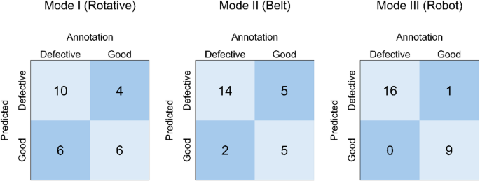
Confusion matrix for different inspection modes.
To complement the sample-by-sample analysis, Table 2 provides a comprehensive comparison across all inspected parts by summarizing the overall part-level performance of the three inspection modes in terms of Recall and F1-score, including 95% bootstrap confidence intervals as a measure of variability.
Table 2 Part-level performance on the test set. Values are point estimates with 95% bootstrap confidence intervals (resampling over parts).
To quantify the uncertainty associated with the part-level confusion-matrix results, Table 2 reports non-parametric bootstrap 95% confidence intervals obtained by resampling the 26 test parts (the same physical parts were inspected under all three modes). On the full test set (Subset: ALL), Robot achieves the highest performance with Recall = 1.00 (95% CI [1.00, 1.00]) and F1 = 0.97 (95% CI [0.89, 1.00]). Belt shows intermediate performance (Recall = 0.88 [0.69, 1.00]; F1 = 0.80 [0.62, 0.92]), while Rotative yields the lowest values (Recall = 0.62 [0.38, 0.86]; F1 = 0.67 [0.43, 0.84]). Although the bootstrap interval is degenerate for Robot recall due to perfect detection on the available test set, this result should be interpreted within the limited sample size and validated on larger production datasets.
Overall, the confidence intervals indicate more robust part-level performance for Robot, whereas Belt and especially Rotative exhibit larger variability across resampled test sets.
These results quantitatively support the ranking previously observed at frame level. Mode I (Rotative) shows the weakest performance, with low precision due to numerous false positives and low recall indicated by many false negatives. In contrast, Mode II (Belt) improves in defect detection, with a noticeable decrease in undetected anomalies. Nonetheless, the best outcomes are achieved with Mode III (Robot), where there is a significant reduction in both undetected defects and wrongly rejected parts, confirming its effectiveness against both false positives and false negatives.
Trajectory optimization
After analyzing the testing results, Mode III exhibited the best defect detection performance and the most robust inspection strategy against false positives. Despite its effectiveness, the adopted strategy is not the most efficient due to the generic camera trajectory used during inspection.
Five new samples with varying defect visibility levels were inspected using Mode III. The detection algorithm was run directly on the inspection video, sampling frames at 200 ms intervals (5 frames per second). Figure 13 shows an example of the inference results for a specific sample.
Fig. 13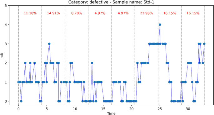
Number of correctly detected defects over time with the robot inspection technique for a specific sample.
The y-axis represents the number of detected defects per frame, while the x-axis shows time. The total video length (30 s) was divided into equal intervals, and the percentage of detected defects per interval was calculated. The percentage of detected defects varies with time, indicating specific camera angles that enhance defects visibility. These results are represented in an interval plot (Fig. 14), showing significant differences among group means, proving that different perspective angles can significantly affect defect visibility.
Based on this analysis, the inspection strategy was optimized. The total inspection time remained fixed, but movements related to the lowest defect detection rate were minimized, and more time was spent on angles with the highest detection rates. Testing parts were then inspected using the optimized strategy, with results reported in Fig. 15.
Fig. 14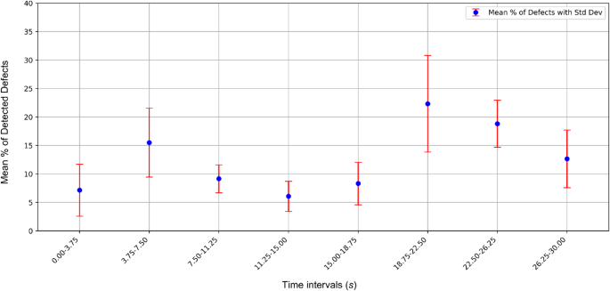
Mean percentage of detected defects per time interval among different samples.
Fig. 15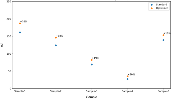
Number of detected defects with the robot inspection for different inspection trajectories.
The graph shows the total number of detected defects per sample for both the original and optimized strategies. The optimized strategy improved the defect detection success rate, with the percentage improvement noted for each sample.
The optimized trajectory was evaluated on a limited subset of five samples. Therefore, these results should be interpreted as preliminary proof-of-concept evidence of feasibility rather than as a statistically general conclusion. A broader evaluation on a larger and more diverse set of parts will be considered in future work.