
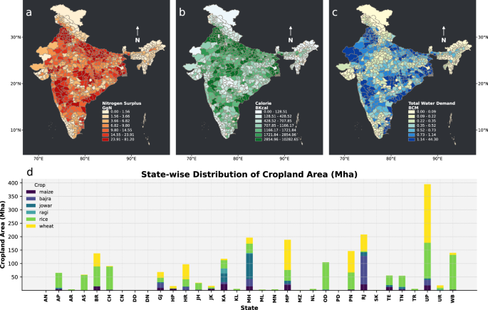
Our study uses a linear multi-objective optimization model to assess cereal-crop restructuring in India. The model reallocates existing district-season cereal area among six focal cereals while minimizing nitrogen surplus and consumptive water demand, preserving state-level calorie production as an energy-availability safeguard, and maintaining benchmarked cereal net return. The workflow integrates district-level crop area and yield data for 1997–2020, crop-specific synthetic fertilizer and manure application rates13,64, atmospheric nitrogen deposition, cropland-level biological nitrogen fixation input terms, state-level crop-specific C2 production-cost benchmarks64, official state-year cereal price benchmarks derived from value-of-output and production statistics, national crop-level realized-price fills for the few unmatched state-crop combinations, and crop calorie values (Supplementary Fig. S1 and Supplementary Tables 1–12). The six modeled cereals are rice (Oryza sativa), maize (Zea mays), wheat (Triticum aestivum), jowar (Sorghum vulgare), bajra (pearl millet), and ragi (finger millet), which together represent most cereal production in India. The different components of our methodology are detailed below.
Resource calculation for baseline scenario
To establish a baseline for our study, we selected 2017 as the reference year65, against which all changes in water, nutrients, benchmarked cereal net return, calories and agricultural greenhouse gas emissions (AGHG) were measured. The choice of the baseline year is mainly determined by the availability and quality of the underlying data. We obtained crop yield and harvested area data for the rabi (non-monsoon) and kharif (monsoon) seasons for the six focal cereals from the Directorate of Economics and Statistics crop-reporting portal66. The dataset includes 664 districts, covering approximately 87% of India’s land area66. The source data report five planting seasons: winter, autumn, kharif, rabi, and summer. For this analysis, winter was grouped with rabi, and summer and autumn were grouped with kharif66. The resulting two-season classification follows the major Indian cropping seasons: kharif (June–October; monsoon) and rabi (November–March; winter). We calculated nitrogen (N) and phosphorus (P) input rates from synthetic fertilizers, manure, the cropland-level BNF input term, and atmospheric deposition. Crop-specific plot-level N and P fertilization rates, together with manure application rates, were obtained from the Government of India’s Cost of Cultivation survey. We adapted the aggregation approach of Davis et al.35 to derive district-level crop-specific fertilizer and manure input rates in kg ha−1. Where district observations were unavailable, state-level crop averages were used; where state-level observations were unavailable, national crop averages were used. The district-level input for district i in state j, crop c, and year t was calculated as:
$${Z}_{i,j,c,t}=\frac{{\sum }_{v}\left({K}_{v,i,j,c,t}\cdot {Z}_{v,i,j,c,t}\right)}{{\sum }_{v}{K}_{v,i,j,c,t}},$$
(1)
where Zv,i,j,c,t is the input amount reported for plot v, and Kv,i,j,c,t is the corresponding cluster weight in the Cost of Cultivation dataset67,68. Manure application rates from the plot data were converted to nitrogen and phosphorus equivalents using uniform nutrient-content factors of 0.5% N and 0.3% P69.
Biological Nitrogen Fixation (BNF) refers to the microbial conversion of atmospheric nitrogen into reactive nitrogen inputs to cropland70. The BNF term used here is the annual cropland nutrient-budget input reported in the FAOSTAT Cropland Nutrient Budget dataset4, harmonized in kg N ha−1 yr−1 and merged by year into the district-crop database. Because the focal crops are cereals, this term represents an exogenous cropland nutrient-budget input, not crop-specific symbiotic fixation by cereal plants. The 2017 baseline optimization applies the same annual FAOSTAT BNF value across the six focal cereals; the adopted value is reported in Supplementary Table 12 and clarified further in Supplementary Methods 3.
The quantification of atmospheric nitrogen (N) deposition, encompassing both dry and wet deposition of NHx and NOy, was derived from atmospheric chemical transport models. We utilized data from the National Center for Atmospheric Research (NCAR), specifically from the Chemistry-Climate Model Initiative (CCMI), which forms part of the input datasets for Model Intercomparison Projects (input4MIPS)71. This dataset provides monthly data from 1850 to 2014, with a spatial resolution of 1.9∘ latitude by 2.5∘ longitude. The data were interpolated to the required district resolution using nearest-neighbor interpolation and aggregated to an annual time step.
Crop nutrient uptake was defined as the nutrient embedded in harvested grain45. We used crop nutrient-content values from Supplementary Table 272 to estimate harvested nutrient output:
$$N{u}_{output(i,j,c,t)}=P{r}_{i,j,c,t}*N{u}_{content(i,j,c,t)}$$
(2)
where Nuoutput(i, j, c, t) represents the nitrogen and phosphorus embedded in the produced crop. Pri,j,c,t is the quantity of crop produced in kg, and Nucontent(i, j, c, t)(kg/kg) represents the nutrient content. Nuoutput is only considered for the part of the produced crop (grain).
District-level N surplus (NS; kg N ha−1 yr−1) and P surplus (PS; kg P ha−1 yr−1) were calculated as applied nutrient inputs minus harvested grain nutrient output72:
$$\begin{array}{l}{{{{\rm{NS}}}}}_{(i,j,c,t)}={N}_{{{{{\rm{DEP}}}}}_{(i,j,t)}}+{N}_{{{{{\rm{FERT}}}}}_{(i,j,c,t)}}+{N}_{{{{{\rm{BNF}}}}}_{t}}\\+{N}_{{{{{\rm{MAN}}}}}_{(i,j,c,t)}}-{N}_{{{{{\rm{output}}}}}_{(i,j,c,t)}}\end{array}$$
(3a)
$${{{{\rm{PS}}}}}_{(i,j,c,t)}={P}_{{{{{\rm{FERT}}}}}_{(i,j,c,t)}}+{P}_{{{{{\rm{MAN}}}}}_{(i,j,c,t)}}-{P}_{{{{{\rm{output}}}}}_{(i,j,c,t)}}$$
(3b)
where NS(i, j, c, t) is the N surplus for crop c in district i and state j in year t; NDEP is atmospheric nitrogen deposition; NFERT and PFERT are synthetic fertilizer inputs; NBNF is the annual cropland-level BNF input term from FAOSTAT; NMAN and PMAN are manure-derived N and P inputs; and Noutput and Poutput are harvested grain nutrient outputs. All terms are expressed per hectare per year in the corresponding nutrient units.
Long-term averages were utilized to fill in missing values for district fertilizer and manure application rates. Leveraging the principle of nutrient mass balance, we estimated the nutrient surplus (Nusur) within the soil, representing the disparity between Nuinput and Nuoutput. This surplus encapsulates nutrients persisting in the soil post-crop production. While a fraction of Nusur is recycled within the soil, a substantial portion is prone to environmental loss, potentially manifesting as nitrogen and phosphorus losses in various forms, such as nitrous oxide emissions into the atmosphere and nitrate and phosphorus leaching into surface and groundwater sources13,38,73. Recognized as an environmental pollution indicator, nutrient surplus also functions as a proxy for virtual nutrient pollution, a measure encompassing the nutrient quantity lost to the environment throughout the entire production cycle of a specific crop commodity39,74. The method for surplus calculation is known to introduce substantial uncertainties globally, owing to variations in estimates of crop nitrogen content, biological nitrogen fixation (BNF), and manure management practices. These factors are documented at various resolutions and detailed in the literature13,75.
We calculated crop-specific total crop water demand (CWD) for 2017 by combining blue and green water components from Kampman et al.76. Following Dalin et al.77, state-level CWD coefficients were adjusted to district-year yield conditions:
$$CW{D}_{i,j,c,s,t}=CW{D}_{j,c,s,2000}\cdot \frac{{Y}_{j,c,s,2000}}{{Y}_{i,j,c,s,t}}$$
(4)
where i, j, c, s, and t denote district, state, crop, season, and year, respectively; CWDi,j,c,s,t is district-level crop water demand; Y is crop yield; and CWDj,c,s,2000 is the Kampman et al.76 state-season crop water-demand coefficient for 2000.
We estimated the benchmarked district cereal net return as sales revenue minus production cost. Production costs use crop-specific state-level C2 cost-of-production benchmarks from the Government of India Agricultural Statistics at a Glance 201764. These values are reported in Rupee quintal−1 and were merged to district observations by state and crop. Specifically, the benchmark uses the source-table cost-of-production entry reported on the C2 basis in Rupee quintal−1, rather than the separate per-hectare cultivation-cost entries. Because no district-level production-cost series is available, the same state-crop C2 benchmark was applied to all districts within a state. The DES C2 concept includes both paid-out costs and imputed owned-resource costs; the relevant cost concepts and source-table fields are summarized in Supplementary Tables 10, 1168, and the operational interpretation is detailed in Supplementary Methods 2. Total district production cost was calculated as:
$$C{p}_{i,j}^{{{{\rm{total}}}}}={\sum}_{c}\left(10\times {\Pr }_{i,j,c}\times C{p}_{j,c}^{{{{\rm{prod}}}}}\right)$$
(5)
where \(C{p}_{i,j}^{{{{\rm{total}}}}}\) is total production cost (Rupee), Pri,j,c is crop production in tonnes, \(C{p}_{j,c}^{{{{\rm{prod}}}}}\) is the state-crop C2 production-cost benchmark in Rupee quintal−1, and the factor of 10 converts tonnes to quintals.
Sales revenue used the 2017–18 benchmark selling price \(S{P}_{j,c}^{{{{\rm{bench}}}}}\) (Rupee quintal−1). For each state-crop combination with a usable official realized price, \(S{P}_{j,c}^{{{{\rm{bench}}}}}\) was calculated as the state-year crop value of output divided by state-year crop production. Where a direct state-crop price was unavailable or unusable, we applied the corresponding all-India crop-level realized price for 2017–18 so that the benchmark retained complete cereal coverage without introducing district-level price imputation. Using realized unit prices reduces the risk that crop-specific differences in actual price realization are obscured by a common national support-price schedule. MSP values are therefore retained as a separate policy-support benchmark, whereas the realized-price series defines the primary revenue input. Supplementary Table 3 reports the MSP reference values, Supplementary Fig. S16 documents realized-price departures from MSP and indicative terms of trade, and Supplementary Figs. S17, S18 provide the district-MSP comparison benchmark. Sales revenue was then calculated as:
$$S{R}_{i,j}={\sum}_{c}\left(10\times S{P}_{j,c}^{{{{\rm{bench}}}}}\times P{r}_{i,j,c}\right)$$
(6)
where SRi,j is district sales revenue (Rupee). The benchmark price is applied uniformly to districts within each state-crop pair because realized prices are available at state-year, not district, resolution.
Benchmarked district cereal net return was calculated as sales revenue minus total production cost28,36:
$${B}_{i,j}=S{R}_{i,j}-C{p}_{i,j}^{{{{\rm{total}}}}}$$
(7)
where Bi,j is benchmarked cereal net return for district i in state j. For the optimization constraint, the corresponding state-crop net-return coefficient is:
$${\pi }_{j,c}=10\left(S{P}_{j,c}^{{{{\rm{bench}}}}}-C{p}_{j,c}^{{{{\rm{prod}}}}}\right),$$
where πj,c is expressed in Rupee tonne−1.
District-level total calorie production (kcal) was computed as:
$${K}_{{{{\rm{cal}}}},i}={\sum}_{c=1}^{n}{\Pr }_{i,c}\times {{{{\rm{kc}}}}}_{c}$$
(8)
Here, Pri,c is crop production in tonnes, and kcc is the calorie density (kcal tonne−1) for crop c (Supplementary Table 4). Within the optimization framework, this calorie term defines a state-level energy-availability floor; broader dietary quality and nutritional security require additional nutrient-specific targets.
Setting up the optimization algorithm
We formulated the crop-restructuring problem as a set of linear optimization models. The decision variable xi,j,c,s denotes the cultivated area allocated to crop c in district i, state j, and season s. Let Dj be the set of districts in state j, C = {rice, wheat, maize, bajra, jowar, ragi}, and S = {rabi, kharif}. The model reallocates the existing district-season cereal area among the six focal cereals, while holding total district-season cereal area fixed and allowing only cereals with historical presence in the district-season crop set. Crop yields, nitrogen-surplus coefficients, water-demand coefficients, calorie densities, and net-return coefficients are treated as fixed 2017 baseline coefficients. The constraints preserve state-season calorie production as an energy-availability floor and maintain benchmarked cereal net return under the 2017–18 revenue benchmark described above. Broader dietary quality and nutritional security are not optimization objectives. For combined annual summaries, optimized Rabi and Kharif outputs are summed after solving the seasonal allocation problem.
We solved two single-objective models, one minimizing nitrogen surplus and one minimizing consumptive water demand, and a multi-objective weighted-sum model that balances the two objectives. For the multi-objective frontier, nitrogen surplus and water demand were normalized by their 2017 baseline totals inside the weighted objective so the two quantities could be combined despite their different units. We report the resulting Pareto frontier in absolute units (Tg N and BCM) and use percentage changes relative to the 2017 baseline for endpoint co-benefit summaries.
A single-objective optimization model was developed to minimize total nitrogen surplus (FN), with cultivated area as the decision variable33. This was achieved while maintaining or enhancing state-level calorie production and benchmarked cereal net return. The nitrogen-surplus objective is:
Objective function:
$$\min \quad {F}_{N}(x)={\sum}_{s\in S}{\sum}_{j}{\sum}_{i\in {D}_{j}}{\sum}_{c\in C}{x}_{i,j,c,s}\,N{S}_{i,j,c,s}$$
(9)
Here, NSi,j,c,s is the per-hectare nitrogen-surplus coefficient (kg N ha−1) for crop c in district i, state j, and season s, calculated from the nitrogen input and harvested-output terms described above.
Constraints:
1.
The total cereal area in each district-season must remain unchanged. This constraint ensures that the optimization reallocates existing cereal cropland rather than expanding or contracting the cultivated area, as shown in equation (10):
$${\sum}_{c\in C}{x}_{i,j,c,s}={\sum}_{c\in C}{A}_{i,j,c,s}^{{{{\rm{cu}}}}}\quad \forall i\in {D}_{j},\,\forall j,\,\forall s\in S$$
(10)
2.
Crop substitution is limited to cereals historically cultivated within a given district, preserving local agronomic plausibility. Feasible crops are defined by the historical-presence indicator:
$${x}_{i,j,c,s}=0\quad {{{\rm{if}}}}\quad {A}_{i,j,c,s}^{{{{\rm{hs}}}}}=0\quad \forall i\in {D}_{j},\,\forall j,\,\forall c\in C,\,\forall s\in S$$
(11)
No crop-specific historical maximum area constraint is imposed beyond the historical-presence rule, because historical crop area reflects past adoption and procurement conditions rather than a strict future ceiling.
3.
Maintaining total calorie production. Total calorie production within each state-season must not fall below the 2017 baseline value, as shown in equation (12). This preserves baseline state-level caloric output as an energy-availability floor during crop restructuring. A nutrient-aware formulation would require additional nutrient-specific targets.
$${\sum}_{i\in {D}_{j}}{\sum}_{c\in C}{{{{\rm{kc}}}}}_{c}\,{x}_{i,j,c,s}\,{Y}_{i,j,c,s}\ge {\sum}_{i\in {D}_{j}}{\sum}_{c\in C}{{{{\rm{kc}}}}}_{c}\,{A}_{i,j,c,s}^{{{{\rm{cu}}}}}\,{Y}_{i,j,c,s}^{{{{\rm{cu}}}}}\quad \forall j,\,\forall s\in S$$
(12)
Here, kcc is the crop-specific calorie density from Supplementary Table 4.
4.
Benchmarked cereal-net-return stability. State-season net return, evaluated with the net-return coefficient πj,c defined above, must not fall below the 2017 baseline. This preserves a net-return floor under the benchmarked price environment:
$${\sum}_{i\in {D}_{j}}{\sum}_{c\in C}{\pi }_{j,c}\,{x}_{i,j,c,s}\,{Y}_{i,j,c,s}\ge {\sum}_{i\in {D}_{j}}{\sum}_{c\in C}{\pi }_{j,c}\,{A}_{i,j,c,s}^{{{{\rm{cu}}}}}\,{Y}_{i,j,c,s}^{{{{\rm{cu}}}}}\quad \forall j,\,\forall s\in S$$
(13)
Here, πj,c is the state-crop net-return coefficient defined above.
This optimization model, with its specified objective function and constraints, provides a structured methodology for analyzing the impact of crop restructuring on nutrient surplus while adhering to land availability, calorie adequacy, and net-return-preservation requirements.
We also set up a single-objective water-demand minimization model using the same constraints. The objective function is:
$$\min \quad {F}_{W}(x)={\sum}_{s\in S}{\sum}_{j}{\sum}_{i\in {D}_{j}}{\sum}_{c\in C}CW{D}_{i,j,c,s}\,{x}_{i,j,c,s}$$
(14)
Here, CWDi,j,c,s denotes the consumptive crop water demand per unit cultivated area. This function minimizes total cereal water demand under the same land, historical-presence, calorie-production, and income-preservation constraints.
The multi-objective optimization framework addresses nitrogen surplus and water demand simultaneously using a weighted objective78,79. The combined objective is:
$$\min \quad \alpha \frac{{F}_{N}(x)}{{F}_{N}^{2017}}+\left(1-\alpha \right)\frac{{F}_{W}(x)}{{F}_{W}^{2017}}$$
(15)
In this formulation, α is a weighting factor ranging from zero to one in 0.01 increments and controls the relative emphasis on minimizing nitrogen surplus versus water demand. \({F}_{N}^{2017}\) and \({F}_{W}^{2017}\) are the corresponding 2017 baseline totals for nitrogen surplus and consumptive water demand, respectively, and are used to normalize the two objective terms before they are combined. A value of α closer to one places greater emphasis on nitrogen-surplus reduction, whereas a value closer to zero prioritizes water-demand reduction. For each α value, we determined an optimal district-level cropping pattern and calculated national totals of nitrogen surplus and water demand. Plotting these totals gives the Pareto frontier for the Indian cereal system.
The constraints applied to this multi-objective optimization model remain consistent with those detailed above. We also calculate endpoint co-benefits for the two single-objective strategies. To compare nitrogen surplus (kg) with consumptive water demand (m3), we use percentage changes relative to the 2017 baseline. For nitrogen-surplus-focused restructuring, the water co-benefit is the percentage reduction in water demand achieved at the nitrogen-focused endpoint. For water-focused restructuring, the nitrogen co-benefit is the percentage reduction in nitrogen surplus achieved at the water-focused endpoint.
Recognizing the indispensable cultural and dietary roles of rice and wheat as staple cereals in India, our optimization model introduces constraints to reflect their importance. These constraints ensure that adjustments to farming patterns aimed at enhancing water efficiency and reducing nitrogen surplus do not disproportionately affect the cultivation of rice and wheat, acknowledging their fundamental place in Indian agriculture and cuisine.
As in the primary optimization framework, these scenarios reallocate crop composition within the baseline district-level cropped area and therefore do not expand or contract total agricultural area. The retained staple-area floor is imposed at the state level, allowing the preserved rice or wheat area to be redistributed among districts within the same state.
We applied this cultural constraint to rice only for the kharif season and to wheat for the rabi season, as these are their primary growing periods in India. The details are as follows:
For rice (r), the constraint ensures that the total rice area retained within each state does not fall below a specified fraction of its current (Acu) state total, represented in equation (16):
$${\sum}_{i\in {D}_{j}}{x}_{i,j,r,{{{\rm{kharif}}}}}\ge \tau {\sum}_{i\in {D}_{j}}{A}_{i,j,r,{{{\rm{kharif}}}}}^{{{{\rm{cu}}}}}\quad \forall j$$
(16)
Similarly equation (17), for wheat (w):
$${\sum}_{i\in {D}_{j}}{x}_{i,j,w,{{{\rm{rabi}}}}}\ge \tau {\sum}_{i\in {D}_{j}}{A}_{i,j,w,{{{\rm{rabi}}}}}^{{{{\rm{cu}}}}}\quad \forall j$$
(17)
Here, τ is a retention parameter ranging from 0 to 1, where τ = 1 preserves the baseline state-level staple crop area and smaller values progressively relax that retained-area requirement while allowing within-state redistribution across districts.
By incorporating these constraints, the model pragmatically balances sustainability objectives with the cultural imperatives of rice and wheat cultivation in India. This approach underscores the complexity of agricultural optimization in contexts where cultural preferences play an important role in shaping dietary patterns.
Implications of optimization on various environmental factors
We evaluated the impact of cropland restructuring across various critical dimensions. First, in the environmental dimension, we compared nitrogen surplus and water minimization strategies, examining greenhouse gas (GHG) emissions, nitrogen loss through leaching/runoff and emissions, phosphorus application, and surplus generation. Second, in the social dimension, we analyzed how the trade network would evolve and be impacted by cropland restructuring aimed at reducing nitrogen surplus. Finally, we examined the economic dimension by calculating the social cost of mitigating nitrogen pollution if nitrogen surplus-based restructuring were implemented in India, highlighting the potential monetary gains at the national level.
We evaluate the percentage change in total greenhouse gas (GHG) emissions relative to the baseline value. GHG emissions are calculated under two scenarios: one where only nitrogen surplus minimization is focused (α = 1) and another where only water consumption minimization is focused (α = 0).
District- and crop-specific agricultural greenhouse gas (AGHG) emissions were quantified by integrating three key sources: (i) methane (CH4) emissions from rice cultivation under distinct water management regimes, (ii) emissions from open-field burning of crop residues, and (iii) nitrous oxide (N2O) emissions derived from nitrogen surplus in croplands.
For each crop c in district i, the total AGHG emissions were expressed as:
$${T}_{{{{{\rm{AGHG}}}}}_{i,c}}={E}_{i,c}^{{{{{\rm{CH}}}}}_{4}}+{E}_{i,c}^{{{{\rm{Burning}}}}}+{E}_{i,c}^{{{{{\rm{N}}}}}_{2}{{{\rm{O}}}}-{{{\rm{surplus}}}}}$$
(19)
where each term is expressed in CO2-equivalent units (CO2eq) per unit cultivated area.
State-level CH4 emission factors for rice were estimated by weighting regime-specific emission coefficients (EFr, kg CH4 ha-1) by the proportion of rice area (ps,r) under each water management regime in state s:
$${E}_{s,{{{\rm{rice}}}}}^{{{{{\rm{CH}}}}}_{4}}={\sum}_{r}\left({p}_{s,r}\times E{F}_{r}\right)$$
(20)
Regimes considered included continuous flooding, single aeration, multiple aeration, upland, deepwater, drought-prone, and flood-prone categories. Area shares were obtained from regional literature80, and regime-wise emission coefficients were sourced from India’s BUR III report and are summarized in Supplementary Table 88. The resulting CH4 emissions were converted to CO2eq using the 100-year global warming potential for CH4 (\(GW{P}_{{{{{\rm{CH}}}}}_{4}}=28\)):
$${E}_{s,{{{\rm{rice}}}}}^{{{{{\rm{CH}}}}}_{4}-{{{{\rm{CO}}}}}_{2}{{{\rm{eq}}}}}={E}_{s,{{{\rm{rice}}}}}^{{{{{\rm{CH}}}}}_{4}}\times 28$$
(21)
The state-level coefficient was then assigned to all rice-producing districts within that state.
Open-field burning emissions for rice, wheat, maize, and millets were estimated following IPCC inventory guidelines and India-specific residue-burning coefficients81,82. The calculation incorporated crop-specific residue-to-crop ratios (RCRc), dry matter fractions (DMFc), state-specific fractions of residue burned (FBs,c), and the fraction actually oxidized (FAO = 0.93). The state-specific FBs,c overrides listed in Supplementary Table 6 follow Jain et al.82, while all remaining cereal-state combinations were assigned the default value of 0.10 used in that inventory. Broader residue and GWP constants are summarized in Supplementary Table 7. Methane and nitrous oxide emission factors (\(E{F}_{{{{{\rm{CH}}}}}_{4}}=2.7\) kg t-1; \(E{F}_{{{{{\rm{CO}}}}}_{2}}=1515\) kg t-1; \(E{F}_{{{{{\rm{N}}}}}_{2}{{{\rm{O}}}}}=0.07\) kg t−1) were obtained81 and are summarized in Supplementary Table 9, while GWPs were taken as \(GW{P}_{{{{{\rm{CO}}}}}_{2}}=1\), \(GW{P}_{{{{{\rm{CH}}}}}_{4}}=28\) and \(GW{P}_{{{{{\rm{N}}}}}_{2}{{{\rm{O}}}}}=265\)83. The per-unit production emission factor was calculated as:
$$\begin{array}{l}E{F}_{s,c}^{{{{\rm{burning}}}}}=RC{R}_{c}\times DM{F}_{c}\times F{B}_{s,c}\times FAO\\ \times \left(E{F}_{{{{{\rm{CH}}}}}_{4}}\times GW{P}_{{{{{\rm{CH}}}}}_{4}}+E{F}_{{{{{\rm{CO}}}}}_{2}}\times GW{P}_{{{{{\rm{CO}}}}}_{2}}+E{F}_{{{{{\rm{N}}}}}_{2}{{{\rm{O}}}}}\times GW{P}_{{{{{\rm{N}}}}}_{2}{{{\rm{O}}}}}\right)\end{array}$$
(22)
Multiplication of \(E{F}_{s,c}^{{{{\rm{burning}}}}}\) by district-level production (Areai,c × Yieldi,c) yielded total district-crop residue-burning emissions; dividing by cultivated area gave the corresponding per-hectare intensity where needed.
Nitrogen surplus for each district and crop was computed as the sum of all nitrogen inputs (synthetic fertilizer, manure, biological fixation, atmospheric deposition) minus nitrogen removal via harvested biomass. State-specific emission fractions (\({f}_{{{{{\rm{N}}}}}_{2}{{{\rm{O}}}},s}\), %) were derived from the IMAGE-GNM global nutrient model55. The resulting N2O emissions (kg ha−1) were calculated as:
$${E}_{i,c}^{{{{{\rm{N}}}}}_{2}{{{\rm{O}}}}-{{{\rm{surplus}}}}}={N}_{{{{{\rm{surplus}}}}}_{i,c}}\times \frac{{f}_{{{{{\rm{N}}}}}_{2}{{{\rm{O}}}},s}}{100}$$
(23)
These were converted to CO2eq using \(GW{P}_{{{{{\rm{N}}}}}_{2}{{{\rm{O}}}}}=265\).
The total AGHG intensity for each district-crop combination was calculated as:
$$\begin{array}{l}GH{G}_{i,c}^{{{{{\rm{CO}}}}}_{2}{{{\rm{eq}}}}}={E}_{i,c}^{{{{{\rm{CH}}}}}_{4}-{{{{\rm{CO}}}}}_{2}{{{\rm{eq}}}}}+{E}_{i,c}^{{{{\rm{Burning}}}}-{{{{\rm{CO}}}}}_{2}{{{\rm{eq}}}}}\\+{E}_{i,c}^{{{{{\rm{N}}}}}_{2}{{{\rm{O}}}}-{{{\rm{surplus}}}}-{{{{\rm{CO}}}}}_{2}{{{\rm{eq}}}}}\end{array}$$
(24)
This framework was applied annually over the study period using year-specific data for crop areas, yields, nitrogen surplus, and water management regime shares where available. The 2017 district-level, crop-specific AGHG intensities (Mg CO2eq ha−1) were subsequently used for the baseline optimization and scenario comparisons.
We calculated the percentage change in nitrogen lost to the environment through leaching/runoff losses (\({{{{\rm{NO}}}}}_{3}^{-}\)) and nitrous oxide loss (N2O-N) relative to baseline values. This nitrogen loss to the environment was calculated under two endpoint scenarios: nitrogen-surplus minimization (α = 1) and water-demand minimization (α = 0). Nitrogen loss was estimated as a fixed fraction of nitrogen surplus (NS), following methods from previous literature38,84. The loss fractions were derived using the dynamic IMAGE-GNM model55 (Supplementary Fig. S15). Nitrous oxide loss was quantified using equation (25):
$${N}_{{{{\rm{N}}}}}2{{{\rm{O}}}}-{{{\rm{N}}}}={\sum}_{j}N{S}_{j}\,E{F}_{j}$$
(25)
Here, NN2O − N represents total national N2O-N loss from surplus nitrogen in managed soils (kg). The emission factor for state j (EFj) was calculated using IMAGE-GNM model data13. Aquatic nitrogen loss through leaching and runoff was calculated as:
$$\begin{array}{r}{N}_{{{{\rm{leach}}}}}={\sum}_{j}N{S}_{j}\,L{F}_{j}\end{array}$$
(26)
In this equation, Nleach represents total nitrogen lost to aquatic systems through leaching and runoff. The leaching fraction for state j (LFj) represents the fraction of nitrogen surplus in managed soils that is lost by leaching and runoff. These coefficients were derived using spatially explicit data from the IMAGE-GNM model13.
We investigated the consequences of nitrogen-surplus-reduction-based crop restructuring on Indian interstate agricultural trade networks at the state level85. District-level optimized crop production was first aggregated to states and then linked to the interstate trade network. We used trade-network data from Kulkarni et al.57 and Goyal et al.13, focusing on the three-year average trade volumes around the 2017 baseline. These data include crop-specific volumes in tonnes for rice and wheat, and aggregate volumes for maize, bajra, jowar, and ragi, which we collectively refer to as alternative cereals. States are represented as nodes, direct exchanges as edges, and edge weights as crop or crop-group trade volumes.
The restructured trade network was calculated from an exporter-centric perspective. For each staple crop k ∈ {rice, wheat}, the baseline export ratio for exporting state i was calculated as ρi,k = Wi,k,2017/Pi,k,2017, where Wi,k,2017 is total baseline exports and Pi,k,2017 is baseline production. If optimization changed production to Pi,k,opt, the optimized export volume was Wi,k,opt = ρi,kPi,k,opt, with link-level exports scaled by the same exporter-specific ratio. When reduced rice and wheat exports created a calorie deficit on a trade link from exporter i to importer j, the staple-calorie deficit was calculated as:
$$\begin{array}{l}{D}_{ij}^{{{{\rm{staple}}}}}=\left({W}_{ij,{{{\rm{rice}}}},2017}-{W}_{ij,{{{\rm{rice}}}},{{{\rm{opt}}}}}\right){{{{\rm{kc}}}}}_{{{{\rm{rice}}}}}\\+\left({W}_{ij,{{{\rm{wheat}}}},2017}-{W}_{ij,{{{\rm{wheat}}}},{{{\rm{opt}}}}}\right){{{{\rm{kc}}}}}_{{{{\rm{wheat}}}}}\end{array}$$
(27)
where i is the exporting state, j is the importing state, W is expressed in tonnes, and kc is the crop-specific calorie density.
For links where optimized staple trade exceeded baseline, \({D}_{ij}^{{{{\rm{staple}}}}}\) was set to zero for the alternative-cereal reconstruction. To compensate for positive staple-calorie deficits, alternative cereals (maize, bajra, jowar, and ragi) were allocated on the union of baseline alternative-cereal links and exporter-importer pairs with positive \({D}_{ij}^{{{{\rm{staple}}}}}\), expressed in kcal. Link strengths for alternative cereals were updated as:
$${W}_{ij,{{{\rm{alt}}}},{{{\rm{opt}}}}}^{{{{\rm{kcal}}}}}={W}_{ij,{{{\rm{alt}}}},2017}^{{{{\rm{kcal}}}}}+{D}_{ij}^{{{{\rm{staple}}}}}$$
(28)
subject to the exporter production-capacity constraint:
$${\sum}_{j=1}^{n}{W}_{ij,{{{\rm{alt}}}},{{{\rm{opt}}}}}^{{{{\rm{kcal}}}}}\le {P}_{i,{{{\rm{alt}}}},{{{\rm{opt}}}}}^{{{{\rm{kcal}}}}}$$
(29)
where \({W}_{ij,{{{\rm{alt}}}},2017}^{{{{\rm{kcal}}}}}\) is the baseline alternative-cereal trade volume converted to kcal and \({P}_{i,{{{\rm{alt}}}},{{{\rm{opt}}}}}^{{{{\rm{kcal}}}}}\) is optimized alternative-cereal production in exporting state i, also expressed in kcal. If a positive staple-deficit link had no baseline alternative-cereal flow, Eq. (28) introduced a new alternative-cereal link on that exporter-importer pair.
This ensures that lost staple calories are compensated on the modeled trade links, while the optimization itself separately enforces state-level calorie and benchmarked-income constraints. The trade-network reconstruction is formulated as a calorie-preserving redistribution exercise; it is not an independent market-equilibrium model for realized export revenue.
We translated the observed reductions in N leaching (\({{{{\rm{NO}}}}}_{3}^{-}\)) and nitrous oxide (N2O) emissions (see eqs. (26), (25)) relative to the baseline year into monetary terms by applying per-kilogram damage costs (USD kg−1 N) for nitrogen losses to water and air, capturing health, ecosystem, and climate damages. All monetary values are reported in constant 2015 USD. Unit costs were taken from Sutton et al.56 (Supplementary Table 5), converted from INR to USD using the World Bank average official exchange rate for 201586, and, where necessary, adjusted to 2015 prices using the World Bank GDP deflator. Costs were scaled to India’s 2015 gross national income87.
Sensitivity and uncertainty analysis
We quantified uncertainty in nutrient surplus and loss estimates derived from fertilizer and manure application data from the Cost of Cultivation survey (2009–2019) for six major crops across all districts of India64. To propagate uncertainty from farmer-reported input use, we implemented nonparametric bootstrapping with 1000 iterations, resampling district-level observations by crop and year. The resulting empirical confidence intervals were propagated to subsequent socio-environmental outcome assessments, including benchmarked cereal net return, agricultural greenhouse-gas (AGHG) emissions, water use, and nitrogen balances, thereby explicitly incorporating input variability into modeled outcomes. For the combined endpoint comparison shown in Fig. 2b, we additionally propagated district-input uncertainty through 500 bootstrap realizations of water-demand and net-nitrogen coefficients, re-solved the two endpoint strategies, and recalculated all ten displayed socio-environmental metrics. Figure 2b reports the national endpoint value together with the 2.5th–97.5th percentile interval of this bootstrap distribution for each displayed metric; the fixed-allocation frontier bootstrap design used for Supplementary Fig. S19 is described in Supplementary Methods 1. Where data availability was limited, or input parameters originated from heterogeneous sources, we performed one-at-a-time sensitivity analyses by perturbing baseline values by ± 10% for benchmarked cereal net return, AGHG emissions, consumptive water use, and nitrogen surplus. Because nitrogen surplus comprises multiple components, including biological nitrogen fixation, atmospheric deposition, manure application, and synthetic fertilizer use, we also varied each component independently by ± 10% to assess their individual influence under data constraints and to identify the relative contribution of each pathway to overall surplus variability. Sensitivity and uncertainty results are reported alongside baseline estimates in Fig. 2b and Supplementary Figs. S7–S11, S19.
Data management and analysis
Data assembly and preprocessing were conducted in Excel 2016 (Microsoft) and Python. Linear programs were solved with the PuLP Python library. Figures and post-optimization summaries were generated in Python and Origin.
Reporting summary
Further information on research design is available in the Nature Portfolio Reporting Summary linked to this article.