
Species distribution data
We used the International Union for Conservation of Nature (IUCN) Red List of Threatened Species database, which provides EOO data for 11,552 extant fish species44. We complemented IUCN EOO data by compiling point occurrence records from a combination of datasets (Supplementary Table 1). We followed the same procedure as IUCN—that is, we merged sub-basin units of the HydroBASINS datasets at level 8 containing one or more point occurrence records of the species45. We included species with at least 10-point occurrence records available in the complementary dataset29. Our analysis focuses on lotic species (that is, those that are found in flowing water bodies). Thus, we excluded lentic species that occur exclusively in stagnant water bodies29. Species are lotic if they were associated with habitats containing at least one of the terms ‘river’, ‘stream’, ‘creek’, ‘canal’ or ‘channel’29. We excluded species if their EOO areas were less than 103 km2 (~10 grid cells). Synonyms were collected from FishBase, IUCN and ref. 46, with accepted species names validated in FishBase. Our final dataset included 9,809 species. We compared species coverage derived from the integrated point-occurrence dataset with the freshwater fish database in ref. 46, compiled at the biogeographic realm scale. This comparison indicates broadly representative global coverage, although species richness in northern Asia remains underestimated (Extended Data Fig. 9).
Water temperature data
We used the global water temperature database, FutureStream, which provides weekly water temperature data at a 5-arcminute spatial resolution generated using global hydrological and water temperature models (PCR-GLOBWB, DynWat)34. These models are driven by climate data from five general circulation models (GFDL-ESM2M, HadGEM2-ES, IPSL-CM5A-LR, MIROC-ESM-CHEM and NorESM1-M), each forced by four RCP emissions scenarios (RCP2.6, RCP4.5, RCP6.0 and RCP8.5) as part of the Coupled Model Intercomparison Project Phase 534. We used a global river network at 5-arcminute spatial resolution, upscaled from the MERIT-Hydro dataset, to provide topological information for grid cells, along with additional hydrologic attributes such as river length47. We chose the MERIT-Hydro (1/12°) river network over the PCR-GLOBWB river-routing network for the analysis because, although both are at the same spatial resolution, MERIT-Hydro is derived from a high-accuracy, hydrologically corrected digital elevation model, ensuring more realistic flow paths and river connectivity. This level of topographic detail is critical for accurately capturing species’ habitat structure and dispersal pathways. In contrast, the PCR-GLOBWB routing network is optimized for hydrological modelling and may oversimplify river topologies and length, making it less suitable for species-level ecological analyses such as TFE. Nonetheless, we note that the choice of drainage network had a minimal impact on TFE, as TFE quantifies species-level climate-induced spatial heterogeneity of warming, rather than pinpointing the exact location of individual suboptimal temperature pixels (Extended Data Fig. 10).
We used high-resolution (1 km) August stream-temperature data for the 1:100,000-scale National Hydrography Dataset Plus, provided by the NorWeST project48. Historical mean August water temperatures spanning 1993–2015 were used to establish the relationship between temperature differences and distance for defining TFE. We selected this regional monthly temperature dataset because it is the only high-resolution water temperature dataset available at the ~1 km river-reach scale, which allows for a more accurate representation of stream network topology and thermal heterogeneity.
Species-specific thresholds for extreme water temperature
We used maximum weekly water temperatures to represent one side of species-realized niche limits. Previous research has suggested that increases in maximum water temperature constitute a larger threat to freshwater fish than changes in minimum water temperature or extreme flow conditions under climate change1. To assess climate change threats to freshwater fish, we focused on maximum rather than mean thermal conditions, as extreme temperatures are more decisive drivers of local extinctions and potential range contractions1,49.
We quantified species-specific thresholds for maximum weekly water temperature based on the extant distribution of water temperatures within species EOOs, similar to previous studies1,10,12. The long-term averaged species-specific weekly maximum temperature threshold was estimated in two steps1. First, we estimated the annual maximum weekly water temperature during 1976–2005 and calculated the mean of the 30-year time-series data for each grid cell. We then overlaid the species’ EOOs with the long-term averaged weekly maximum temperature and considered the 97.5th percentile of the mean annual maximum weekly water temperature within the species’ EOOs as the species-specific thresholds. We used the percentiles rather than absolute maximum values to reduce the influence of uncertainties and outliers in the threshold definition1. To remain more conservative and resistant to outliers in our estimates of species-specific thresholds, we used the 97.5th percentile instead of the more commonly used 95th or 99th percentile to define extreme events. A comparison between our species-specific thresholds and the critical thermal maxima reported in ref. 22 suggests both under- and overestimations, but overall reasonable agreement (mean bias = 9%; Pearson’s r = 0.52; Extended Data Fig. 6). Further comparisons with species-specific thresholds defined at the 95th and 99th percentiles are provided in Supplementary Text 4 and Supplementary Figs. 4 and 5.
Definition of thermal exposure characteristics
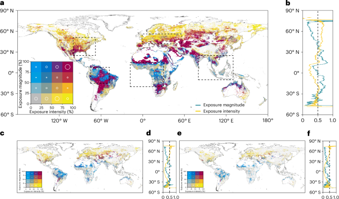
We describe thermal exposure characteristics from four perspectives: thermal exposure intensity, magnitude, abruptness and timing. First, we defined an extreme thermal event as a period during which a species is exposed to temperatures above its species-specific threshold for at least three consecutive weeks (Extended Data Fig. 1). Although the three-week period is arbitrary, studies on a limited set of species suggest that even single-day extreme thermal events can have substantial biological impacts10. Here a three-week duration is chosen to avoid classifying short, transient temperature spikes as ecologically meaningful extremes, as many freshwater fish can buffer short-term exposure through behavioural or physiological acclimation50,51. Moreover, because our species-specific thresholds represent the 97.5th percentile of weekly temperatures within each species’ current ranges, reflecting upper realized thermal conditions rather than acute physiological limits (Extended Data Fig. 6), a multi-week exceedance better captures chronic deviations from each species’ present-day thermal niche. Nevertheless, we also repeated all analyses using 2-, 4- and 6-week duration thresholds, and the overall spatial and statistical patterns remained consistent (Supplementary Figs. 6–8). Since multiple extreme thermal events can occur within a single calendar year, we defined the annual thermal exposure intensity as the maximum temperature observed across all extreme thermal events within the year. The intensity of each extreme thermal event was calculated as the mean of the temperature differences between the species-specific threshold and the weekly water temperatures exceeding that threshold (Extended Data Fig. 1). To complement the short-term effects of extreme thermal exposure, we also quantified the duration and frequency of short-term extreme events. For each species and grid cell, we calculated the annual total number of weeks above the species-specific threshold (duration) in extreme thermal events and the number of extreme thermal events per year (frequency) (Supplementary Figs. 1 and 2). Together with intensity, these metrics reflect the overall severity of short-term thermal stress experienced by species (Supplementary Fig. 3).
To reflect the long-term effects of extreme water temperatures, we introduce the concept of long-term extreme thermal events. If a species experiences at least one short-term extreme thermal event in each year of a 5-year window, we consider the species to be exposed to unprecedented temperatures for a long period. The median of the 5-year exposure period is then taken as the time at which a long-term extreme thermal event occurs. This running-window is applied consecutively across all 5-year periods during 2006–2099. For species that breed annually or near-annually, 5 years represents a considerable number of breeding seasons at temperatures beyond which these species have never been recorded12. This definition does not assume that extreme thermal events coincide with or fully span the breeding season in all species or years, but instead captures chronic, multi-year thermal pressure acting across generations.
Thermal exposure magnitude, abruptness and timing are all calculated based on long-term extreme thermal events (Extended Data Fig. 2). We calculate the cumulative percentage of species in the assemblage that have experienced lasting extreme thermal events over the course of the twenty-first century. In our framework, once a species experiences a long-term extreme thermal exposure event, it is counted as exposed for all subsequent years within that assemblage. First, thermal exposure magnitude is defined as the maximum of the cumulative percentage of species in the assemblage under long-term thermal exposure. Second, the abruptness of exposure for an assemblage was calculated as the percentage of newly exposed species that occur in the decade of maximum exposure relative to the exposure magnitude. Third, we identified the exposure abruptness timing as the midpoint in the decade of maximum exposure. Abruptness and timing were calculated only for assemblages in which five or more species were exposed, to avoid idiosyncrasies due to small sample sizes12,52. Species not exposed before the end of the twenty-first century were excluded from this calculation.
Definition of TFE
We introduce the concept of temperature distance (Lj,i,s, in kilometres) to represent the thermal cost for species s when travelling through river reach i within river segment j. A river reach is defined relative to the spatial resolution of the underlying water temperature dataset, representing the smallest unit to which a water temperature attribute is assigned. A river segment represents a dendritic network composed of a cluster of connected river reaches. The core idea behind temperature distance is to reflect the thermal cost species may encounter when moving through a river network under rising temperatures. Our assumption is that reaches where temperatures exceed species-specific thresholds function as thermal barriers and impose thermal costs, with higher exceedance corresponding to higher thermal cost. Previous analysis focusing on landscape climate connectivity has directly established a linear relationship between thermal cost and temperature difference by setting temperature distance weight as a constant37,53. Here we used the space-for-time method to establish a relationship between temperature distance (Lj,i,s) and temperature difference along time (Lj,i,s, in °C) (Supplementary Text 5):
$${L}_{j,i,s}=f\left({\Delta T}_{\mathrm{time}}\right)$$
(1)
To reflect the thermal cost for each species, ∆Ttime is defined as the temperature difference between future scenarios (Tsc;j,i,s) and species-specific threshold (Tthreshold;s), which represents thermal exposure intensity as defined in thermal exposure characteristics:
$$\begin{array}{l}\Delta T_{\mathrm{time}}={T}_{\mathrm{sc}{{;}}j,i,s}-{T}_{\mathrm{threshold}{{;}}s}\left({T}_{\mathrm{sc}{{;}}j,i,s} > {T}_{\mathrm{threshold}{{;}}s}\right);\\\qquad\qquad\Delta T_{\mathrm{time}}=0\left({T}_{\mathrm{sc}{{;}}j,i,s}\le {T}_{\mathrm{threshold}{{;}}s}\right)\end{array}$$
(2)
where Tsc;j,i,s is the temperature of river reach i within river segment j under future scenarios connected with the habitat of species s. Under the assumption of space-for-time, temporal thermal gradients (ΔTtime) are represented by the spatial thermal gradients, expressed as the absolute temperature differences (∆T) between river reaches i and m within the same river segment j (noted as \({T}_{{i}_{\!j}}\) and \({T}_{{m}_{\!j}}\)):
$$\Delta T=|{T}_{{i}_{\!j}}-{T}_{{m}_{\!j}}|{ \sim \Delta T}_{\rm{time}}$$
(3)
To present the relationship between temperature difference (ΔT) and river-reach distance between river reaches i and m within the river segment j (\({D}_{\!j}^{i,m}\)), we used August stream-temperature data from the NorWeST project, which provides water temperature data at the river-reach scale with 1 km resolution. \({D}_{\!j}^{i,m}\) are computed as the cumulative river-reach length summed along the flow path (watercourse distances), using the geometric properties of the National Hydrography Dataset Plus network adopted by the NorWeST project. This high-resolution, regional vector-based river network allowed us to calibrate the parameters a and b:
$$\Delta T=a{\left({D}_{\!j}^{i,m}\right)}^{b}$$
(4)
The median ∆T between reaches i and m within segment j, along with their river-reach distance (\({D}_{\!j}^{i,m}\)), was fitted using a non-linear power function. The resulting exponents were a = 0.85 and b = 0.24. The representativeness of the ΔT–D relationship and parameters uncertainty and sensitivity are discussed in Supplementary Text 6 (Supplementary Figs. 9–14).
Based on the space-for-time method, the temperature distance Lj,i,s can be interpreted from river-reach distance \({D}_{\!j}^{i,m}\), and ΔTtime is represented as a thermal cost expressed in distance units (Lj,i,s). Due to the convex shape of the fitted function, temperature distance responds less sensitively to early-stage warming compared to later periods, making this approach more conservative than previous analyses37,53.
An empirical dispersal kernel \(k\left(L\right)\) defined as a probability density function was adopted to explain the probability of successful dispersal over a given distance54:
$$k\left(L\right)=C\frac{p}{{\uppi }u{\left(1+\frac{{L}^{2}}{u}\right)}^{p+1}}$$
(5)
$$K\left(L\ge x\right)={\int }_{x}^{\inf }k\left(L\right)$$
(6)
Here L represents the temperature distance (Lj,i,s) in kilometres, k is the empirical dispersal kernel and p = 0.18 and u = 550 are movement parameters provided in ref. 54 and validated using comprehensive empirical data on species distributions in the Mississippi River basin55. The parameters in the dispersal kernel have also been applied in regions such as the Indian Peninsula, where species distribution data are insufficient for independent calibration54. We further discuss the sensitivity of this parameter set and its ecological interpretation in Supplementary Text 7 and 8 (Supplementary Figs. 15–18) (C = 320.57 is determined numerically such that \(K\left(x\ge 0\right)=1\)).
Note that the \(K\left(L\right)\) does not vanish, even for long distance. Therefore, a threshold B0 is considered to represent thermal block—that is, interactions of populations from the species are completely blocked when the probability is lower than B0. In this study, we set B0 = 0.1 as the thermal block threshold to incorporate abrupt changes:
$${B}_{j,i,s}={K}_{j,i,s}{{;}}\,{B}_{{j},{i},{s}}=0\left({K}_{{j},{i},{s}} < {B}_{0}\right)$$
(7)
where Kj,i,s is the probability of species s going through the temperature distance Lj,i,s, and Bj,i,s is the truncation of Kj,i,s after considering B0. Blocking probability is defined as 1 − Bj,i,s, representing the intensity of thermal exposure on a scale from 0 to 1. The sensitivity of B0 is discussed in Supplementary Text 9 (Supplementary Figs. 19 and 20).
For each species s, TFE is developed based on ref. 1, by multiplying Bj,i,s as a weight factor:
$${\mathrm{TFE}}=1\,-\,\frac{{\sum }_{i=1}^{N}{\left({\sum }_{j=1}^{M}{B}_{{j},{i},{s}}{d}_{j,i,s}\right)}^{2}}{{\sum }_{i=1}^{n}\left({{\sum }_{j=1}^{m}{d}_{j,i,s}}\right)^{2}}$$
(8)
where n and N are numbers of river segments within the geographic range of species s; m and M are numbers of river reach within the segment i for species s and dj,i,s is the length of river reach.
Partitioning the causes of TFE change
The factors driving changes in TFE can be grouped into four categories based on whether suboptimal temperatures occur in the historical or future period, and whether the affected reaches lie inside or outside a species’ EOO (Extended Data Fig. 4). First, we identified river reaches that already exhibited suboptimal temperatures during the historical period, representing habitats that are naturally thermally isolated. Second, we considered river reaches that will be suboptimal due to climate-driven temperature changes. Third, we distinguished suboptimal conditions occurring within a species’ geographic range (‘in EOO’). Finally, we accounted for suboptimal temperatures in reaches located outside of a species’ range but connecting habitat patches (‘out EOO’).
To isolate the contribution of climate change to TFE (∆TFE), we calculate the difference between TFE during 2006–2099 and the mean TFE from 1976 to 2005. We define ∆TFE > 20% as indicative of high risk, as nearly 96% of species are projected to experience mean ΔTFE values during 2006–2035 below this level relative to the historical baseline (1976–2005) under the RCP2.6 scenario. To quantify the extra effect of TFE occurring in river reaches outside of EOO but connecting habitat patches (TFEout), we assume these reaches are always optimal and calculate the TFE based on this assumption (TFEin). The difference between TFE and TFEin is then used to estimate TFEout. We do not instead assume that reaches inside the EOO are always optimal to calculate TFEout, because reaches within the EOO are inherently the priority for conservation.
Our approach highlights the significance of managing river-reach temperatures outside species’ current ranges, particularly during early periods of warming when temperatures within EOOs may still be suitable. Three representative species with potamodromous, resident and anadromous life-history strategies were selected to map their EOOs and illustrate how warming shifts thermal blocks that affect TFE and TFEin values (Extended Data Figs. 7 and 8 and Supplementary Text 2).
TFE trajectory classification
We adopted the classification framework proposed in ref. 56. Both linear and non-linear models were fitted to compare the resulting classifications of TFE trajectories. Four statistical models were applied to each time series. Linear models were categorized into two types: ‘linear’ (a1 ≠ 0, a2 = 0) for those with a significant trend (p values < 0.05), and ‘no-trend’ (a1 = a2 = 0) for those without a significant trend. For non-linear modelling, we used a second-order polynomial model (a2 ≠ 0) to capture the non-linear shape of the trajectory over time56,57,58, and a step model to identify ‘abrupt’ changes. All classification codes are provided in ref. 56.
According to the trajectory shape, the function f followed one of the following forms:
$$f\left(t\right)={a}_{2}{t}^{2}+{a}_{1}t+{a}_{0}+\varepsilon \left(t\right)$$
(9)
$$f\left(t\right)={a}_{0}+{\beta }_{0}I\left(t > e\right)+\varepsilon\left(t\right)$$
(10)
where a0, a1, a2 and β0 are coefficients of the models and e is the threshold parameter, with I(t > e) = 1 when t > e and 0 otherwise.
We adjusted the interval size parameter (δ ∈ [0,1]) governing directional classification from the default value of 0.5 to 0.3 for quadratic trajectories. This modification requires consistent slope signs within the midpoint (Xm ± 15% of the series length, rather than ±25% previously) to classify trends as ‘increase’ or ‘decrease’; otherwise, trends are classified as ‘stable’. The original value of 0.5 for δ was designed to minimize the false detection of trends by using half of the time series to decide the change direction58. However, this also requires trajectories to change quickly at the early stage, which could lead to the misclassification to ‘stable concave’ when the trajectory includes a prolonged stable period followed by a later, more pronounced increase—a pattern commonly seen in the TFE pattern under RCP8.5. By reducing the interval size to 0.3, the method becomes more sensitive to delayed accelerations and improves the detection of these characteristic TFE patterns. Meanwhile, it ensures that the trajectory direction remains constant for at least 65% of the total timespan, which we consider sufficient to capture its main direction.
Temporal autocorrelation
The temporal autocorrelation of TFE was quantified by calculating the spectral exponent. We performed spectral analysis using periodograms derived from fast Fourier transforms to assess the power associated with each frequency in the detrended TFE24,25. The spectral exponent was calculated as the slope of the linear regression between the log-transformed power and the log-transformed frequency. A more negative slope indicates stronger temporal autocorrelation, meaning that the time series is primarily influenced by low-frequency variations.
Reporting summary
Further information on research design is available in the Nature Portfolio Reporting Summary linked to this article.