
Improved mass balance representation through daily glacier modelling
In our daily configuration (hereafter, “daily model”), GloGEM resolves surface mass balance at a daily time step using daily temperature and precipitation. In contrast, in the standard monthly GloGEM configuration, surface mass balance is computed from monthly mean temperature and total monthly precipitation, with precipitation phase based on monthly temperature and melt estimated using a statistical approach that represents sub-monthly temperature variability using the monthly standard deviation of daily temperatures derived from historical data16,36 (see “Methods”). While this monthly formulation (hereafter, “monthly model”) allows melt to occur in months with mean temperatures below 0 °C, it does not explicitly resolve daily temperature variability (Supplementary Fig. 1).
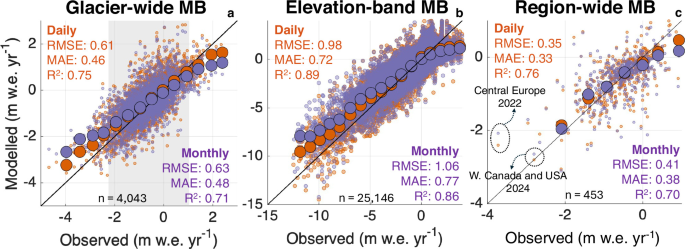
We first evaluate model performance by comparing annual climatic mass balances from the daily and monthly models with 4037 independent glacier-wide annual in situ observations37. For this evaluation, all glaciers with available observations are included, rather than restricting the analysis to the >5 km2 subset used for the global projections. In general, the daily model shows a slight improvement over the monthly model with the root mean squared error (RMSE) decreasing from 0.63 to 0.61 m w.e., the mean absolute error (MAE) decreasing from 0.48 to 0.46 m w.e., and the coefficient of determination (R2) increasing from 0.71 to 0.75 (Fig. 1a). These skill scores also represent an improvement over earlier evaluations of GloGEM16 (RMSE: 0.73 m w.e), which were based on fewer glaciers, shorter records, and lacked glacier-specific calibration data14. At the regional scale, however, improvements are not uniform (Supplementary Fig. 2 and Supplementary Table 2). Most regions show similar or improved performance for the daily model, while others show little change or slightly degraded skill metrics, reflecting regional calibration uncertainties, differences in climate regimes, and limited observational coverage. Regions with sparse mass-balance observations, such as the Russian Arctic and New Zealand, provide only limited opportunities for robust model evaluation, highlighting the continued need for long-term in situ observations in underrepresented glacier regions.
Fig. 1: Comparison of modelled and observed glacier mass balance (MB) for the daily and monthly models using the cross-calibrated parameter configuration.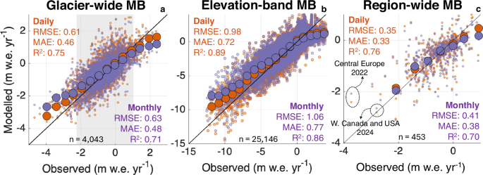
a Modelled versus observed glacier-wide annual specific mass balance over the period 1980–202437. Only glaciers with at least three years of observations are included (175 glaciers). The larger circles show the mean mass balance within bins of 0.5 m w.e. to better isolate the signal. The grey area shows the mean observed mass balance ±2σ. The number (n) of comparisons is indicated at the bottom of each panel. b As in panel a, but evaluated across glacier elevation bands. c Mean annual modelled region-wide mass balance compared to observations between 2000 and 20241. The comparison relies on observational estimates that include all glaciers, whereas our simulations are restricted to glaciers larger than 5 km2. The larger circles show the mean within bins of 0.5 m w.e., where more than three values are available.
Given that uncertainties in annual WGMS mass-balance observations38 are typically of the order of ~0.2-0.4 m w.e. yr−1, the improvement in overall RMSE and MAE should be regarded as modest. The added value of the daily model becomes more apparent in extreme years. For mass-balance anomalies outside ±2σ from the mean, the RMSE decreases from 0.98 to 0.83 m w.e, and the MAE decreases from 0.81 to 0.64 m w.e, when moving from the monthly to the daily model. This indicates a substantially improved representation of both strongly negative and strongly positive mass balance years, driven by enhanced sensitivity to short-term meteorological extremes and steeper mass balance gradients (Supplementary Fig. 3).
Similar improvements are found for mass balances aggregated over elevation bands and for regional mass changes (Fig. 1b, c). The higher RMSE for the elevation-band values is expected, as these data provide a more detailed test of the vertical mass-balance distribution, whereas calibration is primarily constrained by glacier-wide geodetic mass balances (see “Methods”). For the regional comparison, differences in spatial coverage should be kept in mind, as our simulations are restricted to glaciers >5 km2 while the GlaMBIE estimates1 represent the full regional glacier inventory. Nevertheless, the improvement with daily rather than monthly forcing remains apparent, particularly for extreme mass-balance years.
Since both our daily and monthly glacier models are calibrated against glacier-specific geodetic mass balances for 2000–201939, they are expected to produce nearly identical cumulative mass changes over this period. However, the daily model captures interannual variability more accurately, particularly during extreme years. In the European Alps, for instance, which were subject to several extreme melt years over the past two decades25,40, switching from monthly to daily forcing reduces the RMSE of regional mass balances over 2000–2024 from 0.48 to 0.42 m w.e. compared to GlaMBIE observations1. During the record Alpine melt year of 2022, the daily model simulates a mass balance that is 0.31 m w.e. more negative than the monthly model, which is substantially closer to observations (Fig. 1c). Comparable improvements for the daily model are found for other recent extremes, including daily-monthly differences of 0.15 m w.e. in Western Canada and the USA in 202341 and up to 0.98 m w.e. in Svalbard in 202442. In high-latitude regions, the standard monthly model configuration of GloGEM shows strong biases during extreme melt years (see also the Svalbard region in Supplementary Fig. 2), highlighting the importance of resolving short-lived but climatically decisive events that are smoothed when using temporally aggregated forcing.
The role of daily modelling in glacier runoff timing and composition
Glacier runoff integrates mass-balance processes over time and represents the primary pathway through which glacier change affects downstream hydrological systems. Modelled runoff therefore forms the main interface between glacier models and hydrological and land-surface models, which typically operate at (sub-)daily time steps32,43. Building on the mass-balance differences and variability identified above, we assess how temporal resolution influences modelled glacier runoff timing and composition. Glacier runoff is defined as the sum of ice melt, snow melt and liquid precipitation over the initially glacierised area44, minus refreezing (see “Methods”). We assume that, once generated, all surface water runs off immediately, without temporary storage or delayed release.
In our monthly model, glacier runoff is assumed to be distributed uniformly within each month, resulting in stepped runoff curves that obscure short-term variability (Fig. 2a–d, other regions in Supplementary Fig. 6). In contrast, the daily model explicitly resolves sub-monthly variability in glacier runoff, producing a continuous seasonal cycle (Fig. 2a–d). This enables identification of the timing of high flow (annual maximum) and its temporal evolution. By 2100, for example, the daily model projects high-flow glacier runoff in Western Canada and the USA to occur ~46 days earlier under both Shared Socioeconomic Pathway (SSP) 3–7.0 and SSP5-8.5, relative to the 2001–2020 historical baseline (Fig. 2a). In the Southern Andes, high-flow timing shifts by ~10–40 days earlier, depending on the scenario (Fig. 2c). The monthly model misrepresents these shifts by approximately 15 days. Furthermore, the daily model captures pronounced day-to-day fluctuations in glacier runoff associated with hydrological extremes (e.g., heatwaves and cold spells; see the example for Central Europe in Supplementary Fig. 7b), which are smoothed out in our monthly configuration.
Fig. 2: Evolution and variability of glacier runoff as unravelled through daily modelling.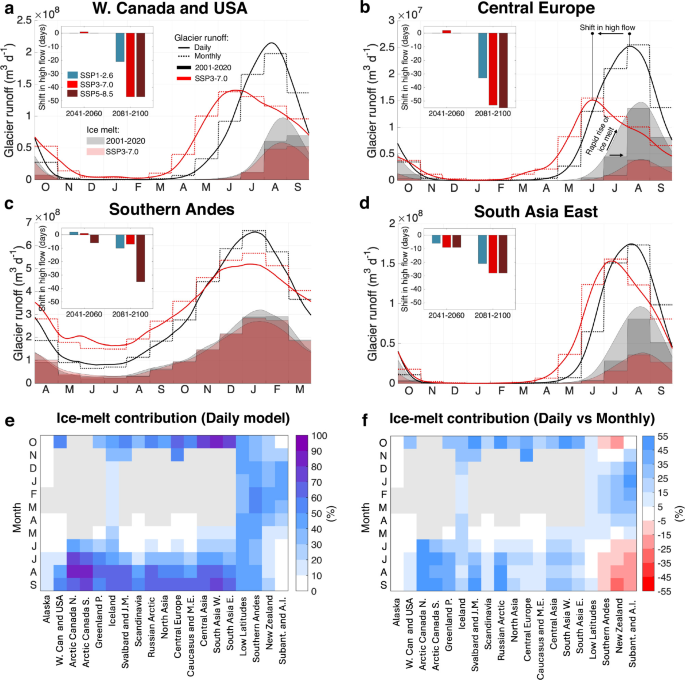
a–d Modelled mean glacier runoff at daily (solid lines) and monthly (dashed lines) resolution for four climatologically distinct regions (panels) (other regions in Supplementary Fig. 6). Shaded areas indicate the ice-melt component of runoff at present-day (grey, 2001–2020) and 2081–2100 under SSP3-7.0 (red). Insets in the top left show shifts in the timing of the seasonal peak (in days) for the daily model compared to the 2001–2020 baseline. e Seasonal cycle of the ice-melt contribution (%) as modelled by the daily model across all RGI regions. Months for which the runoff is <1% of the maximum monthly runoff are greyed out to avoid showing excessively large ice-melt contributions for periods with minimal glacier runoff. f The difference in contribution of ice-melt compared to the monthly model (%).
The temporal resolution also affects the glacier-runoff composition through differences in the frequency at which the surface type is updated within the model. In the daily model, surface transitions (for example, from snow to ice) can occur from day to day in response to melt or snowfall. In contrast, in the monthly GloGEM model, the surface type remains fixed for each month. This generally reduces the modelled summer ice melt contributions in early summer and increases them in latesummer (Fig. 2a–d and Supplementary Fig. 6). Although projected ice melt over the coming decades is therefore lower in the monthly model in many regions, the larger ice volumes remaining by the end of the century (Figs. 3 and 4) eventually lead to greater glacier runoff and ice-melt contributions than in the daily model. As for glacier mass balance, resolving daily meteorological variability leads to stronger interannual variations in simulated glacier runoff. In Central Europe, runoff during the extreme melt year 2022 is 8% higher in the daily model than in the monthly model, whereas runoff is 12% lower during the relatively cool year 2014 (Supplementary Fig. 7a). Across 2000–2024, the median annual daily-minus-monthly runoff difference is −2%, with a standard deviation of 4.5%. These contrasts show that both runoff magnitude and timing are sensitive to year-to-year climate variability and to an explicit representation of sub-monthly processes, especially during extreme years.
Fig. 3: Differences in regional glacier volume projections arising from the transition from monthly to daily modelling, and their underlying drivers.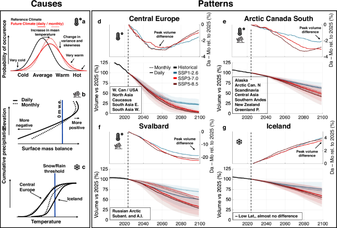
a–c Key processes driving the regional contrasts. The symbols next to each panel letter are repeated in panels d–g to indicate the dominant drivers of the projected daily–monthly differences. The snowflake icon is taken from https://github.com/siemens/ix-icons. Copyright © 2019–2025 Siemens AG. This project is MIT licensed. The temperature icon is taken from Dazzle UI, Dazzle Line Icons collection (CC Attribution License; SVG Repo). d–g Glacier volume projections for four representative regions, each exemplifying a distinct divergence between outputs from the daily and monthly models (regions listed in the boxes in the bottom left follow the same pattern, shown in Supplementary Fig. 9 for every region). In each panel, the lower half represents the multi-GCM mean, and the coloured areas represent ±1 standard deviation, indicating the ensemble spread across GCMs. The upper half highlights the difference in modelled volume between the daily and monthly models, with Da − Mo denoting daily minus monthly simulations and values expressed relative to the 2025 volume.
Fig. 4: Modelled global ice volume evolution, contribution to sea-level rise, and differences between the daily and monthly models.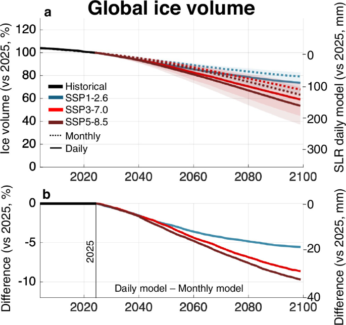
a 21st-century ice volume evolution under different scenarios and the corresponding contribution to sea-level rise (multi-model mean ±1 standard deviation). b Relative difference in ice-volume loss and absolute difference in contribution to sea-level rise since 2025 between the daily and monthly models .
Finally, the explicit separation of snow melt, ice melt and rainfall at daily resolution enables a detailed assessment of the seasonal evolution of glacier-runoff components (Fig. 2). While a similar decomposition is possible in the monthly configuration, interpretation in the latter case is constrained by temporal averaging and the assumed fixed within-month surface states. For instance, for High Mountain Asia (RGI regions 13–15), the daily model shows that ice melt accounts for approximately 70–80% of present-day glacier runoff by late summer (September), whereas the monthly model yields a substantially lower contribution of 44%. In high-latitude regions, ice-melt contributions are much larger in the daily configuration (Fig. 2f). These component-specific runoff estimates are intended as model-based diagnostics of temporal-resolution effects, rather than as directly validated regional partitioning estimates.
Regional and global differences in projected ice volume changes
Beyond its influence on mass balance and runoff variability, the temporal resolution also affects the long-term evolution of projected ice volume (Fig. 3, Supplementary Fig. 9, and Supplementary Table 3). These volume differences mainly arise from differences in climate forcing and model structure, which first affect the simulated surface mass balance (Supplementary Fig. 8) and then accumulate through time into differences in glacier geometry, area and volume. At the regional scale, differences in the 21st-century ice-volume evolution between the daily and monthly models can be grouped into four main patterns (Fig. 3d–g). These patterns consist of differences in timing, persistence, and magnitude of ice volume evolution between the two configurations and mainly reflect regional contrasts in climate variability, glacier hypsometry and elevation range. We refer to these patterns below as (1) transient divergence, with convergence towards deglaciation, (2) persistent divergence in regions with sustained ice cover, (3) amplified divergence in low-relief ice-cap regions, and (4) reversed divergence associated with precipitation-phase effects.
The first pattern is characterised by a transient divergence in ice volume between the daily and monthly models that peaks around mid-century and declines afterward (Fig. 3d). This behaviour is observed in mid-latitude regions with relatively limited present-day ice volumes, such as North Asia, Central Europe, and the Caucasus. In these regions, the daily model typically projects 1–4% greater ice loss by 2050 (relative to 2025), a difference that primarily reflects more negative mass balances under climate change, resulting in accelerated glacier loss (Fig. 3a). However, differences tend to decline thereafter due to rapid deglaciation. Projections from both the daily and the monthly models converge toward near-zero ice volumes by 2100.
The second pattern appears for regions that retain a substantial ice volume throughout the 21st century and therefore exhibit a persistent and, in some cases, increasing divergence between the daily and monthly models (Fig. 3e). This behaviour is observed in regions such as Alaska, Scandinavia, and the Southern Andes, where resolving daily variability produces steeper mass-balance gradients (Supplementary Fig. 3). The latter leads to enhanced mass turnover and a more rapid glacier response to climatic forcing45,46. In addition, the daily model produces more negative annual mass balances (Supplementary Figs. 2 and 8). While these effects accumulate over time, the differences in modelled ice volume remain generally moderate. By the end of the century, the daily model typically projects 2-5% more ice-volume loss than the monthly model, expressed relative to the 2025 glacier volume (Fig. 3e). New Zealand also exhibits enhanced ice loss in the daily model, although this does not appear to be associated with a systematically steeper mass-balance gradient (Supplementary Fig. 3).
The projected amplified glacier loss for the daily model is even more pronounced for Svalbard, the Russian Arctic and the Antarctic and Sub-Antarctic glaciers (Fig. 3f; third pattern). In these low-relief, ice-cap-dominated regions, the narrow elevation range strongly enhances the sensitivity to surface-type transitions and melt-albedo feedbacks, which are further intensified by accelerated warming and the increasing frequency of extreme events associated with Arctic Amplification47. Resolving these processes at daily timescales produces markedly steeper mass-balance gradients (Fig. 3b and Supplementary Fig. 3), more negative mass balances (Supplementary Figs. 2 and 8) and substantially greater ice loss. For these regions, the daily model projects up to ~15% greater relative ice loss over 2025–2060 (vs. monthly model), reaching ~20–25% over 2025–2100 (Fig. 3f). These values should be interpreted as upper-end estimates, as these regions are particularly sensitive to calibration choices (see “Methods” and Supplementary Figs. 4 and 5). These differences are also more pronounced than for other high-latitude regions, such as Arctic Canada North, Arctic Canada South and Greenland periphery (Fig. 3e), where the slightly broader elevation ranges and weaker surface-type feedbacks limit the steepening of mass-balance gradients (for daily vs. monthly model).
Iceland, by contrast, is the only region exhibiting reversed divergence associated with precipitation-phase effects (Fig. 3g; fourth pattern). In this case, the daily model projects 4% less ice loss than the monthly model by 2100. The smaller ice loss in the daily model results from the specific precipitation regime, where heavy precipitation events frequently coincide with relatively warm conditions, as mild south-westerly air masses typically deliver both heat and moisture from the North Atlantic48. In contrast, colder periods dominated by northerly flow are generally drier. Resolving these co-occurrences at daily timescales results in precipitation being classified more often as rain rather than snow (Fig. 3c), reducing snow accumulation. Monthly averaging smooths over these warm events, overestimates the fraction of precipitation falling as snow, and thus overestimates accumulation. This bias propagates into calibration, yielding parameters that slightly increase glacier mass-balance sensitivity to future warming (see “Methods” and Supplementary Figs. 4 and 5).
We further tested the sensitivity of the volume projections to the calibration design by repeating the projections with an alternative calibration setup (the original, independent setup, in which Cprec, Tbias and the DDFs are calibrated separately for the daily and monthly models, see “Methods”). This experiment yields similar or slightly smaller daily–monthly differences, while the regional 21st-century volume changes remain broadly consistent (Supplementary Fig. 10). This indicates that the main regional patterns described above are robust to the choice of calibration strategy.
While a direct comparison with existing global-scale glacier projections from the Climate Model Intercomparison Project version 6 (CMIP6) is complicated by to differences in the choice of the reanalysis product49, future forcing (i.e., a different CMIP6 global climate model (GCM) ensemble considered), model setup, and exclusion of glaciers smaller than 5 km2, there is generally good agreement between values reported in the literature13,14 and projections from our monthly-model (Supplementary Fig. 11). The slightly smaller losses projected by our monthly model compared to previous GloGEM CMIP6 results likely reflect differences in the selected GCM ensemble and the use of an extended reanalysis period up to 2024, which affects the reference state. Updated calibration choices and the >5 km² glacier subset may also contribute, but are unlikely to dominate as we capture the majority of the ice volume (see Supplementary Table 1). The Antarctic and Sub-Antarctic glaciers form a notable exception, for which both the daily and the monthly models project substantially smaller volume losses than reported in previous global assessments, especially under SSP5-8.5. Here, projected differences are particularly sensitive to the representation of surface climate in the reanalysis forcing and of frontal ablation49,50,51, highlighting that forcing and model uncertainty can outweigh temporal-resolution effects in cold, low-melt regimes. In contrast, for Svalbard and the Russian Arctic, our projections are more negative than in previous assessments and are also sensitive to calibration strategy (Supplementary Fig. 10). The magnitude of projected daily–monthly differences in these polar and subpolar regions should therefore be interpreted with care, even though the sign and overall pattern of the temporal-resolution effect remain robust.
Building on the analyses above, we quantify the impact of temporal resolution on projections of global glacier volume. Relative to 2025, our daily model projects global ice losses of 26 ± 10% (SSP1-2.6) and 47 ± 17% (SSP5-8.5) by 2100. Compared with the monthly model, this corresponds to an additional global ice loss of 4–5% by mid-century, increasing to 5–10% by 2100, depending on the scenario (Fig. 4 and Supplementary Table 3). In absolute terms, this implies that the daily model yields 7–15% less global glacier ice remaining by the end of the century compared to the monthly model. The divergence between daily and monthly projections increases steadily throughout the 21st century and does not stabilise by 2100 (Fig. 4b). Given the strong trend still apparent at the end of the century, and previous studies highlighting the multi-centennial response timescales involved in global glacier evolution19,52, these temporal-resolution effects are likely to persist beyond the 21st century. A direct comparison with global CMIP6-based projections remains challenging due to differences in model configuration, including the choice of GCM ensembles and reanalysis data. Nevertheless, our daily model indicates slightly greater 21st-century volume loss than previous CMIP6-based projections14, whereas our monthly configuration yields slightly less loss (Supplementary Table 4).
Implications for large-scale glacier modelling and impacts
The temporal resolution of glacier models is more than a technical choice: it can shape both projected glacier change and its downstream impacts. This is particularly relevant when glacier projections are used in coupled hydrological, land-surface, and impact-assessment frameworks, where the timing, variability and extremes of glacier melt can matter as much as long-term changes in glacier volume. Daily glacier models can explicitly represent nonlinear responses associated with temperature thresholds, short-lived meteorological extremes and rapid surface-state transitions, whereas monthly models generally represent these processes in an aggregated way. Our results show that these differences can propagate into runoff seasonality, interannual variability and long-term ice-volume evolution. Temporal resolution should therefore be considered carefully in impact assessments such as studies of (dry-season) water supply3,34 or hydropower production in glacier-fed catchments.
Adopting daily resolution at the global scale, however, comes with substantial computational costs: in our simulations, resolving daily variability increases processing time substantially compared with monthly simulations (see “Methods”). Although continued increases in computational capacity and model development will likely alleviate these constraints, monthly models will probably remain the standard for many applications in the near term, particularly those focused on large ensembles or probabilistic assessments. The key challenge is therefore not choosing between daily and monthly models but balancing physical realism with computational feasibility according to the addressed question.
In this study, we identified several mechanisms affecting glacier projections that provide potential pathways for improving monthly models. Assumptions of stationary sub-monthly temperature variability based on reanalysis data (see “Methods”) are increasingly inconsistent with observed changes in the variance of temperature distributions under climate change36,53,54,55. Accounting for such non-stationarity would require daily GCM output or other robust information on future changes in sub-monthly temperature variability, to be readily available; however, this is not always the case for all models, scenarios or long-term projection experiments. Likewise, accumulation schemes based solely on monthly mean temperatures misrepresent snowfall where precipitation frequently coincides with warm conditions, as illustrated by the Iceland example. In an additional sensitivity experiment for Iceland, we ran the monthly GloGEM model with accumulation determined from the daily temperature evolution, while the remaining monthly model structure was left unchanged (Supplementary Fig. 12). In that case, the resulting ice-volume evolution shifts much closer to the daily model, confirming that precipitation-phase partitioning is the main driver of the reversed daily–monthly divergence in Iceland (see Fig. 3g). This suggests that relatively simple corrections for sub-monthly temperature variability and precipitation-phase partitioning could improve monthly glacier projections. Refining these components may therefore reduce some of the structural biases associated with temporal aggregation, although their robustness under changing climatic conditions remains uncertain. In parallel, the growing availability of new observational constraints, such as snowlines or snow cover datasets56, provides new opportunities to better constrain the spatial extent of snow cover in glacier models. This could help reduce some of the biases present in glacier models, e.g., those linked to model equifinality, where different parameter combinations can reproduce similar observations18. For the daily version of GloGEM, such observations are particularly promising because remotely sensed daily snow-cover patterns can be compared directly with simulated snow conditions and used as additional calibration or validation constraints57. By contrast, observations representing specific points in time are more difficult to incorporate consistently in a monthly model framework.
In a warming climate marked by more frequent extremes, low-temporal-resolution modelling suppresses short-term variability, which can result in a systematic underestimation of glacier loss. By resolving daily meteorological variability, our simulations consistently project more glacier mass loss than the current monthly GloGEM configuration across most regions, highlighting the potential importance of temporal resolution for downstream impacts. By 2100, our daily model projects a global glacier contribution of 86–157 mm to global mean sea-level rise, exceeding monthly estimates by 20–33 mm (Fig. 4a, b). This additional contribution in the daily model is substantial, although it remains within the GCM ensemble spread shown in Fig. 4a. These additional centimeters resulting from the transition to daily modelling could have direct implications for exposure to coastal flooding, erosion and saltwater intrusion58. As such, our findings indicate that temporal resolution is not a technical detail but a modelling choice with direct consequences for impact assessments. Future glacier projection efforts should therefore explicitly consider temporal resolution, which, combined with informed choices regarding bias correction of climate data59, climate forcing6,49 and calibration strategies60,61,62, will help produce robust and policy-relevant projections of glacier change in a warming world.