Giant orbital Zeeman effects in a magnetic topological van der Waals interphase

Density functional theory

The orbital magnetization in three-dimensional k-space is given by ref. 10

$${{\bf{M}}}^{{\rm{BO}}}= \dfrac{e}{2\hslash}{{\rm{Im}}}{\sum }_{n}\int_{{\rm{BZ}}}\dfrac{d{{\bf{k}}}}{\left(2\pi \right)^{3}}\,{f}_{n{{\bf{k}}}}\left\langle {\partial}_{{\bf{k}}}{u}_{n{{\bf{k}}}}\right\vert \times \left({\hat{H}}_{{\bf{k}}}+{\varepsilon}_{n{{\bf{k}}}}-2\mu \right)\\ \left\vert {\partial}_{{\bf{k}}}{u}_{n{{\bf{k}}}}\right\rangle,$$

(2)

where \(\left\vert {u}_{n{{\bf{k}}}}\right\rangle\) is the Bloch-like eigenstate associated with the nth eigenvalue εnk of the Hamiltonian Hk of the system, fnk is the zero-temperature Fermi occupation factor and μ the chemical potential. Note that the vector product is taken between the two derivatives \({\partial }_{{{\bf{k}}}}=\frac{\partial }{\partial {{\bf{k}}}}\) in the bra and ket, respectively.

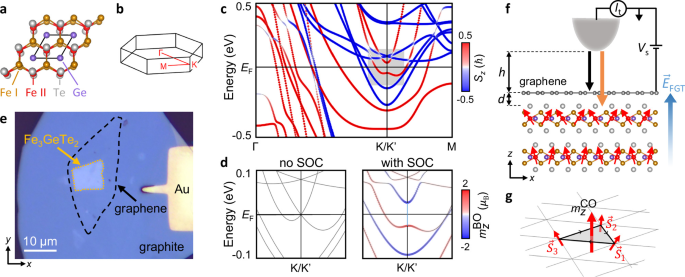
Unlike transport, which probes all occupied states and is therefore sensitive to the orbital magnetization, STM/S probes the either filled or empty states at a given energy and is thus sensitive to the orbital magnetic moment (OMM) of the bands, which is given by

$${m}_{n}{({{\bf{k}}})}^{{{\rm{BO}}}}=\dfrac{e}{2\hslash }{{\rm{Im}}}\langle {\partial }_{{{\bf{k}}}}{u}_{n{{\bf{k}}}}| \times \left({\hat{H}}_{{{\bf{k}}}}-{\varepsilon }_{n{{\bf{k}}}}\right)| {\partial }_{{{\bf{k}}}}{u}_{n{{\bf{k}}}}\rangle .$$

(3)

To calculate this quantity using ab initio methods, we performed the following procedure: The electronic structure of bulk Fe3GeTe2 was computed with the density functional theory code FLEUR52 using the full-potential linearized augmented plane wave method53. We chose the Perdew-Burke-Ernzerhof exchange correlation functional within the generalized gradient approximation54. The FGT lattice parameters are a = 3.99 Å and c = 16.33 Å in a hexagonal close-packed lattice55. We performed a full self-consistent calculation to find the charge density including the effect of spin-orbit coupling within FLEUR, with a resulting magnetocrystalline anisotropy of 1.06 meV per Fe atom. The plane-wave cutoffs for the basis functions, for the charge density and for the exchange correlation functional were set to \(5{a}_{0}^{-1}\), \(15{a}_{0}^{-1}\), and \(12.5{a}_{0}^{-1}\), respectively, where a0 is the Bohr radius. For Fe and Ge, the maximum in the angular momentum expansion was set to \({l}_{\max }=8\) and the muffin-tin radii rMT for both species was set to 2.12a0; for Te, \({l}_{\max }=10\) and rMT = 2.74 a0. Despite previous work on FGT indicating the effects of strong electronic correlations7,12, in the present scenario we do not see indications of such correlations, e.g., as the conduction band minimum is moved through the Fermi energy, and thus did not consider them theoretically. Using the Wannier90 package56,57, from the DFT-calculated Bloch wave functions \(\left\vert {u}_{n{{\bf{k}}}}\right\rangle\), we constructed maximally localized Wannier functions (MLWFs) and determine the Bloch-like basis \(\left\vert {u}_{n{{\bf{k}}}}^{{{\rm{W}}}}\right\rangle\)58,59. A mesh of 8 × 8 × 8 k-points was used with 192 Bloch states to obtain 96 MLWFs. Initial projections were chosen to be d states for Fe and p states for Ge and Te atoms. The maximum frozen window was set to 2.344 eV above the Fermi energy. The Hamiltonian, spin, and orbital angular momentum (OAM) operators were evaluated in the Bloch basis and transformed into the MLWF basis. The OAM was integrated inside the muffin-tins. Further details of the calculations can be found in Ref. 60.

In the Wannier description, the orbital magnetization can be quantified as proposed by Lopez et al.59: First, the Bloch-like basis \(\left\vert {u}_{n{{\bf{k}}}}^{{{\rm{W}}}}\right\rangle\) is transformed into the so called Hamiltonian gauge, using the transformation

$$\left\vert {u}_{n{{\bf{k}}}}^{{{\rm{H}}}}\right\rangle=\mathop{\sum}\limits_{m}^{J}\left\vert {u}_{m{{\bf{k}}}}^{{{\rm{W}}}}\right\rangle {U}_{mn}\left({{\bf{k}}}\right).$$

(4)

This is necessary in order to compute the magnetization according to the so-called “modern theory of orbital magnetization” expression Eq. (2). This expression allowed us to decompose the orbital magnetization into its local

$${{{\bf{M}}}}_{{{\rm{LC}}}}^{{{\rm{BO}}}}=\dfrac{e}{2\hslash }{{\rm{Im}}}\mathop{\sum}\limits_{n}\int_{{{\rm{BZ}}}}\dfrac{d{{\bf{k}}}}{{\left(2\pi \right)}^{3}}\,{f}_{n{{\bf{k}}}}\langle {\partial }_{{{\bf{k}}}}{u}_{n{{\bf{k}}}}^{{{\rm{H}}}}| \times \left({\hat{H}}_{{{\bf{k}}}}-\mu \right)| {\partial }_{{{\bf{k}}}}{u}_{n{{\bf{k}}}}^{{{\rm{H}}}}\rangle,$$

(5)

and itinerant contributions

$${{{\bf{M}}}}_{{{\rm{IC}}}}^{{{\rm{BO}}}}=\dfrac{e}{2\hslash }{{\rm{Im}}}\mathop{\sum}\limits_{n}\int_{{{\rm{BZ}}}}\dfrac{d{{\bf{k}}}}{{\left(2\pi \right)}^{3}}\,{f}_{n{{\bf{k}}}}\langle {\partial }_{{{\bf{k}}}}{u}_{n{{\bf{k}}}}^{{{\rm{H}}}}| \times \left({\varepsilon }_{n{{\bf{k}}}}-\mu \right)| {\partial }_{{{\bf{k}}}}{u}_{n{{\bf{k}}}}^{{{\rm{H}}}}\rangle .$$

(6)

We computed the band-resolved contributions to the magnetization

$${m}_{n,{{\rm{LC}}}}^{{{\rm{BO}}}}=\dfrac{e}{2\hslash }{{\rm{Im}}}\langle {\partial }_{{{\bf{k}}}}{u}_{n{{\bf{k}}}}^{{{\rm{H}}}}| \times \left({\hat{H}}_{{{\bf{k}}}}-\mu \right)| {\partial }_{{{\bf{k}}}}{u}_{n{{\bf{k}}}}^{{{\rm{H}}}}\rangle,$$

(7)

and

$${m}_{n,{{\rm{IC}}}}^{{{\rm{BO}}}}=\dfrac{e}{2\hslash }{{\rm{Im}}}\langle {\partial }_{{{\bf{k}}}}{u}_{n{{\bf{k}}}}^{{{\rm{H}}}}| \times \left({\varepsilon }_{n{{\bf{k}}}}-\mu \right)| {\partial }_{{{\bf{k}}}}{u}_{n{{\bf{k}}}}^{{{\rm{H}}}}\rangle,$$

(8)

similar to ref. 59, where it was shown that Eqs. (5) and (6) can be recast into a gauge-invariant formulation. A more detailed theoretical description will be presented in a forthcoming publication. Finally the orbital magnetic moments in Eq. (3) were determined from the k-resolved local and itinerant contributions as \({m}_{n}{({{\bf{k}}})}^{\rm{BO}}={m}_{n,{\rm{LC}}}^{\rm{BO}}({\bf{k}}) – {m}_{n,{\rm{IC}}}^{\rm{BO}}({\bf{k}})\).

We note at this point that an earlier proposed model of the relevant bands at K/K’9, when inserted into Eq. (3), results in orbital moments which directly contradict our DFT calculations, indicating that such a model does not seem suitable to capture the full orbital physics.

Sample fabrication

Graphite and FGT crystals were exfoliated onto SiO2 and assembled by a standard dry-transfer technique with a microdome polyvinylchlorid/polydimethylsiloxane (PVC/PDMS) stamp61. In the resulting heterostructure, the encapsulation of FGT by the larger graphene and graphite flake prevents the former’s degradation. Ti/Au contacts were fabricated using maskless optical lithography, and samples were subsequently cleaned in an ambient-condition atomic force microscope by repeated scanning in contact mode overnight. Supplementary Fig. S9 shows an AFM image, recorded before the STM measurements, of the heterostructure displayed in Fig. 1e. After introduction into the STM ultra-high vacuum chamber, the sample was annealed at 240 ∘C for 15 min to desorb residues and water and subsequently transferred to the STM. There, the sample was zero-field cooled to the base temperature of ∼6.1 K, and magnetized by ramping the surface-normal field to B = 2 T, prior to STS measurements.

Graphite and Fe3GeTe2 were obtained from commercial sources (graphite from HQ graphene, FGT from 2D semiconductors). FGT bulk crystals from the same batch were characterized by angle-resolved photoemission spectroscopy (ARPES), showing general agreement with the DFT calculations and literature, and a doping level for which EF is close to the topological gap (Supplementary Fig. S8b). STM/S spectra taken on the bulk crystals did not exhibit any peak features and virtually no magnetic field dependence (Supplementary Fig. S8a), confirming the graphene/FGT interface as the source of the observed behavior.

Scanning tunneling experiments

All STM/STS measurements were performed in a commercial Sigma Polar instrument at ∼6.1 K. Electro-chemically etched W tips were annealed to orange glow in vacuum and prepared on an Ag(111) surface. After introducing the heterostructure sample to the STM scanner, we first approached the tip to the contact leads using visual control and then navigated the tip to the heterostructure by scanning. On the heterostructure, we performed large-area STM scans to locate the graphene and FGT flakes and to check the cleanliness of the heterostructure surface. To ensure a clean tunneling spectrum, we then moved the tip back to the Ti/Au contact and safeguarded that it showed a linear I(V) characteristics by repeated careful indentation. We then retracted the tip out of tunneling contact and jumped directly back to the clean surface of the heterostructure, where we performed the measurements, thus preventing any tip alterations that may otherwise occur during intermediate scans. All spectroscopy measurements were performed after ramping the magnetic field above the saturation field of the FGT flake, to achieve a well-defined magnetization. STS was performed using standard lock-in techniques at a frequency of 877 Hz and modulation amplitudes of \({V}_{{{\rm{s}}}}^{{{\rm{mod}}}}=1\,{{\rm{to}}}\,\,3\) meV. STM topographs were analyzed using Gwyddion62.

The trapezoidal shape of the biased tunneling barrier in the WKB-approximation results in a non-linear dependence of the tunneling conductance as the voltage is increased:

$$dI/dV\propto \rho \,{e}^{-2\kappa (E)z},$$

(9)

with the density of states ρ, the decay constant

$$\kappa (E)=\sqrt{\dfrac{2m}{{\hslash }^{2}}({\Phi}_{\rm{eff}} – E)+{k}_{\parallel }^{2}},$$

(10)

the effective barrier height

$${{{\Phi }}}_{{{\rm{eff}}}}=\dfrac{{{{\Phi }}}_{{{\rm{tip}}}}+{{{\Phi }}}_{{{\rm{sample}}}}}{2}$$

(11)

for tunneling bias E = eVs ≪ Φeff, and the momentum in the surface plane k∥. As a result, states close to EF tend to have a smaller dI/dV intensity than those at higher bias. In graphene, the intensity difference between states at lower and higher tunneling bias is further enhanced by the inelastic tunneling channels that become available at ∣eV∣ > ℏω = Eph, which significantly increase the tunneling probability22. Inside this inelastic gap, the elastic tunneling current to the graphene is small, such that tunneling from the FGT dominates: Although the FGT is further away from the tip than the graphene and thus has lower tunneling probability (Eq. (9)), because of its significantly higher density of states compared to the graphene, it dominates the tunneling for ∣eV∣ < Eph: We estimate the respective elastic tunneling probabilities by evaluating Eqs. (9-11) at the Fermi energy (E = 0). For graphene (k∥ = 1.7 Å−1 and z = h = 10 Å), it results e−2κh ≈ 3 × 10−18. For FGT on the other hand (k∥ = 1.05 Å−1 and z = h + d = 13.34 Å), it results e−2κ(h+d) ≈ 5 × 10−18. Thus, the theoretical elastic tunneling probability to the K/K’-point states in the FGT is larger than in the graphene. In addition, since FGT has a significantly higher density of states than graphene, because the Fe 3d bands near K/K’ are flatter than the graphene π-bands, we conclude that the tunneling inside the inelastic gap is dominated by the FGT.

We further note that, because the graphene is in direct contact to the extended metallic FGT flake, dynamical Coulomb blockade effects are strongly suppressed in our experiments63 and thus cannot explain our observed gap features. This argument is supported by the fact that the observed inelastic gaps are almost identical compared to graphene on insulating substrates22,24,26.

The combined observation of a finite peak splitting at zero field followed by an approximately linear shift as function of magnetic field effectively rules out Landau level formation in the graphene as a potential origin of the peak features, since they would follow a square-root dependence \(E\propto \sqrt{B}\) in the absence of lateral confinement64. We expect lateral confinement to be weak in our heterostructure, because the graphene is coupled to the metallic FGT, which renders it n-doped everywhere. Furthermore, our observations are not consistent with conventional quantum-dot (QD) bound states or whispering gallery modes (WGMs): Such states typically give rise to a series of peaks in the density of states corresponding to bound states with increasing (angular) momentum quantum numbers65,66. In contrast, our heterostructure exhibits only two well-isolated peak features within the inelastic gap. These features instead are phenomenologically much more similar to tunable orbital moments of a gapped graphene Dirac cone67,68. In those works, lateral carrier confinement in electrostatically defined potential wells lifts the graphene’s inversion symmetry and gives rise to orbital magnetic moments, which couple to external electric and magnetic fields. In contrast to this work however, in our heterostructure, both, inversion and time-reversal symmetry are already broken, such that we do not require lateral confinement to realize field tunable orbital moments. Instead, we observe the orbital moments of the gapped FGT nodal line, which dominates the tunneling. This interpretation is supported by the fact that the states intrinsic to the graphene shift according to the graphene doping level68, whereas the peaks in our experiments do not: In Fig. 4a, we demonstrate that the graphene doping level can be tuned by ΔED ∼ 15 meV, by changing the tip-sample distance. However, the peaks inside the inelastic gap only shift asymmetrically by ≲ 1 meV, which points to their origin not in the graphene, but in the FGT. This interpretation is again consistent with our argument above, that tunneling inside the inelastic gap is dominated by the FGT. Lastly, we rule out the formation of a quantum dot in the FGT itself, because of its metallic nature.

We extracted ED in Fig. 4a from the V-shaped Dirac spectrum outside the inelastic gap by (i) subtracting the energy offset resulting from the inelastic tunneling process above the phonon threshold ±ℏω, for positive and negative bias voltages separately, and (ii) performing linear fits to the electron and hole sides of the linear Dirac cone spectrum, respectively; the Dirac point energy ED at each setpoint current was then extracted from their intersection. To determine δh in Fig. 4, we used the exponential dependence of the tunneling current on the tip-sample distance \(I/{I}_{0}=\exp (\frac{{h}_{0}-h}{\lambda })\), where δh = h0 − h and λ−1 ≈ (0.455 Å)−1 is the decay constant of the tunneling current for monolayer graphene above the phonon threshold22. Then

$$\delta h=\lambda \ln (I/{I}_{0}),$$

(12)

which is independent of the absolute values of h and h0.

Electrostatic model

From the experimental geometry, we estimate the tip and FGT capacitance density with respect to the graphene as

$${C}_{{{\rm{tip}}}}=\dfrac{{\varepsilon }_{0}}{h}\approx 0.88\,\upmu {\rm{Fc{m}}}^{-2}$$

(13)

$${C}_{{{\rm{FGT}}}}=\dfrac{{\varepsilon }_{0}}{d}\approx 2.651\,\upmu {\rm{Fc{m}}}^{-2},$$

(14)

where ε0 is the vacuum permittivity and we estimate a graphene/FGT layer spacing of d = 3.34 Å and the initial tip height of h = 10 Å at setpoint Vs = 300 mV, I0 = 0.1 nA. We note that, realistically, the permittivity of the graphene/FGT interface is expected to be higher than ε0, which would result in an increase of CFGT and thus a decrease of the electric field at the graphene/FGT interface. The finite screening length of the electric field in the FGT, on the other hand, leads to a decrease of CFGT; however, this change is expected to be small because of the metallic character of FGT and the resulting short screening length69. In any case, both of these effects have only minor influence on the tip-height dependence of the interface field in our study, because the response of the system is dominated by the change of the tip-sample capacitance Ctip.

To model the charge distribution across the junction and the heterostructure, we must take into account that the graphene screens the tip electric field from the FGT, similar to a Faraday screen70. We therefore employed a capacitor model of the junction similar to the one used in ref. 71. Because of the low density of states of graphene close to the Dirac point, the model needs to include the graphene quantum capacitance (per unit sample area)72

$${C}_{{{\rm{q}}}}={e}^{2}\rho,$$

(15)

where

$$\rho=\dfrac{2{E}_{{{\rm{D}}}}}{\pi {(\hslash {v}_{{{\rm{F}}}})}^{2}}$$

(16)

is the spin- and valley-degenerate graphene density of states at EF (per unit sample area), and vF the Dirac Fermi velocity. Integrating ρ from the Dirac point to EF, one obtains from Eq. (16) the number of carriers per unit area in graphene as \({n}_{{{\rm{gr}}}}={\pi }^{-1}{({E}_{{{\rm{D}}}}/\hslash {v}_{{{\rm{F}}}})}^{2}\). As usual, the quantum capacitance is implemented as a capacitor in series to the geometric capacitance between tip and graphene, Ctip (see inset Fig. 4b)71. As a result of the quantum capacitance, the tip electric field is not perfectly screened by the graphene and can penetrate to the FGT underneath, establishing a capacitance CFGT between graphene and FGT, in series with Ctip. Because it is equivalent to a single capacitor with distance h + d, the arrangement of Ctip and CFGT in series is consistent with a tunneling path from the tip directly to the FGT. We thus have two parallel tunneling paths (the other one from the tip to graphene), which suggests putting the two capacitances Cq and CFGT in parallel, both connected to the same back contact of the Ti/Au substrate (within the metallic FGT layer, there will be no potential drop, despite its considerable thickness). In this model, we neglect the inhomogeneity of the electric field due to the curved tip shape, because we are interested only in the properties right underneath the tip apex and the small graphene-FGT distance compared to the tip radius (10–100 nm) results in effectively parallel electric field lines there.

From the circuit diagram it is clear that

$$\dfrac{{n}_{{{\rm{FGT}}}}e}{{C}_{{{\rm{FGT}}}}}=\dfrac{{n}_{{{\rm{gr}}}}e}{{C}_{{{\rm{q}}}}}=\dfrac{{n}_{{{\rm{tip}}}}e}{{C}_{{{\rm{tip}}}}}-{V}_{{{\rm{ts}}}}$$

(17)

and

$${n}_{{{\rm{tip}}}}+{n}_{{{\rm{gr}}}}+{n}_{{{\rm{FGT}}}}=0,$$

(18)

the latter due to charge conservation, where ngr, ntip, and nFGT are the areal charge densities on graphene and the surfaces of the tip and FGT, respectively. We solve the linear equation system by substituting expressions derived from Eq. (17) into Eq. (18), obtaining

$${n}_{{{\rm{gr}}}}+\dfrac{{C}_{{{\rm{tip}}}}{V}_{{{\rm{ts}}}}}{e}+\dfrac{{C}_{{{\rm{tip}}}}}{{C}_{{{\rm{q}}}}}{n}_{{{\rm{gr}}}}+\dfrac{{C}_{{{\rm{FGT}}}}}{{C}_{{{\rm{q}}}}}{n}_{{{\rm{gr}}}}=0.$$

(19)

Using the graphene quantum capacitance (Eqs. (15) and (16))72

$${C}_{{{\rm{q}}}}=\dfrac{2{e}^{2}}{\sqrt{\pi {(\hslash {v}_{{{\rm{F}}}})}^{2}}}\sqrt{{n}_{{{\rm{gr}}}}},$$

(20)

results in

$${n}_{{{\rm{gr}}}}+({C}_{{{\rm{tip}}}}+{C}_{{{\rm{FGT}}}})\dfrac{\sqrt{\pi {(\hslash {v}_{{{\rm{F}}}})}^{2}}}{2{e}^{2}}\sqrt{{n}_{{{\rm{gr}}}}}+\dfrac{{C}_{{{\rm{tip}}}}{V}_{{{\rm{ts}}}}}{e}=0.$$

(21)

Substituting \(a\equiv \frac{\sqrt{\pi {(\hslash {v}_{{{\rm{F}}}})}^{2}}}{2{e}^{2}}\) gives

$${n}_{{{\rm{gr}}}}+a({C}_{{{\rm{tip}}}}+{C}_{{{\rm{FGT}}}})\sqrt{{n}_{{{\rm{gr}}}}}+\dfrac{{C}_{{{\rm{tip}}}}{V}_{{{\rm{ts}}}}}{e}=0,$$

(22)

which yields

$$\sqrt{{n}_{{{\rm{gr}}}}}= -\dfrac{a({C}_{{{\rm{tip}}}}+{C}_{{{\rm{FGT}}}})}{2}\\ +\sqrt{{\left(\dfrac{a({C}_{{{\rm{tip}}}}+{C}_{{{\rm{FGT}}}})}{2}\right)}^{2}-\dfrac{{C}_{{{\rm{tip}}}}{V}_{{{\rm{ts}}}}}{e}},$$

(23)

where only the positive solution of the quadratic expression is physical, as ngr must vanish at Vts = 0. With Eq. (23), we determined the Dirac point energy as

$${E}_{{{\rm{D}}}}=\pm {2e}^{2}a\sqrt{{n}_{{{\rm{gr}}}}}.$$

(24)

The positive (negative) sign applies to holes (electrons).

The potential difference Vts between the tip and graphene is given by the sum of the applied bias voltage and the contact potential difference between tip and sample surface

$${V}_{\rm{ts}}={V}_{\rm{s}}+{V}_{\rm{CPD}}={V}_{\rm{s}}+({\Phi}_{\rm{tip}} – {\Phi}_{\rm{gr}})/e$$

(25)

where the Φ are the respective work functions. While the work function of charge-neutral graphene is well known (see above), the work function of the tip is more difficult to estimate, and critically depends on the details of the tip apex. As a result, for W tips the tip work function typically varies in the range 4.5−5.1 eV11. We indent our W tips into Au before measurements and expect Au to stick to the tip as a result of the preparation procedure. The work function of bulk Au is ΦAu ≈ 5.1 eV, such that we estimate the resulting tip work function to be in the range Φtip = 4.6 −5.1 eV, i.e., greater or equal to that of graphene. The fit in Fig. 4b results in a tip work function of Φtip = (4.66 ± 0.03) eV, in excellent agreement with this range of expected values. Our model further compares well with experiments on graphene/NbSe2 heterostructures (\({\Phi}_{{\rm{NbSe}}_{2}}\) ≈ 5.6 eV), where a significant hole doping corresponding to ED ≈ +400 meV was reported73.

Angle-resolved photoemission spectroscopy

Photoemission measurements were performed on cleaved FGT bulk single crystals and were conducted at NanoESCA beamline at Elettra, using the modified Focus GmbH NanoESCA momentum microscope. The sample was cooled using LHe and the temperature was stabilized at ≈40K. The light was incident at an angle 65° with respect to the surface normal, along the K-Γ-K’ direction. Supplementary Fig. S8b shows spectra collected at ℏν = 60 eV in sweep mode with an energy step size of 0.02 eV.

Disentangling band orbital and chiral orbital Zeeman effects

We approximate the observed peak shifting behavior as function of magnetic field by the linear equation system

$${E}_{1}={g}_{1}{\mu }_{B}B+{E}_{1}^{0}=({g}_{z}^{{{\rm{CO}}}}-{g}_{z}^{{{\rm{BO}}}}){\mu }_{{{\rm{B}}}}B+{E}_{1}^{0}$$

(26)

$${E}_{2}={g}_{2}{\mu }_{B}B+{E}_{2}^{0}=({g}_{z}^{{{\rm{CO}}}}+{g}_{z}^{{{\rm{BO}}}}){\mu }_{{{\rm{B}}}}B+{E}_{2}^{0},$$

(27)

where Ei(B) are the peak energies, with \({E}_{i}^{0}\equiv {E}_{i}(B=0)\), and \({g}_{z}^{{{\rm{CO}}}}\) and \({g}_{z}^{{{\rm{BO}}}}\) are the chiral and band orbital g-factors, respectively. Inserting the fitted slopes from Fig. 3c, g1μB = 1.8 meV/T and g2μB = 13.3 meV/T, results in

$${g}_{z}^{{{\rm{BO}}}}=\dfrac{{g}_{2}-{g}_{1}}{2}\approx 100$$

(28)

and \({g}_{z}^{{{\rm{CO}}}}\approx 130\).