
Data description
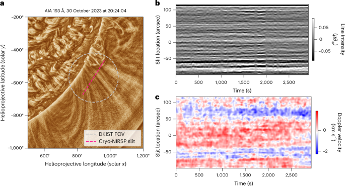
The data were obtained on 30 October 2023 by the Cryo-NIRSP instrument located at the US National Science Foundation’s DKIST. Cryo-NIRSP can observe the corona with a spatial sampling of ~0.12″ (~87 km) along the slit and with temporal cadences of 1 s. The Cryo-NIRSP data used here are a sit-and-stare observation using the 0.5″-wide spectrograph slit with 0.12″ spatial sampling along the slit. The spatial resolution of Cryo-NIRSP is optical-limited to around 0.3″ and seems to be seeing-limited to 0.6″ (due to terrestrial atmospheric seeing)50.
The Cryo-NIRSP instrument was tuned to examine the 1,074.7 nm (iron Xiii) coronal emission line and provided high-quality spectra with a spectral dispersion of 4.4 × 10⁻¹² m per pixel and a resolving power of R ≈ 48,000. The solar spectrum was observed between 1,072 nm and 1,076 nm. This line has been extensively used to probe coronal dynamics14,17,18,19,53 and is resolved well by Cryo-NIRSP51. Supplementary Figs. 1 and 2 contain an example spectrum and the corresponding fits to the line profile, along with a discussion on the measurement uncertainty associated with the Doppler velocities.
The target region for the observations was centred on (X, Y) = (898″, −568″) (a height of 0.1R☉ above the limb). The pointing stability of the data was assessed by examining the motions of the fine structure, and it seems to be ≲0.1″. Hence, the stability of the pointing was better than the estimated seeing resolution along the slit. Further information about the dataset can be found in ref. 50.
Data processing
High-frequency noise in the data can lead to issues when identifying the fine-scale coronal structures. The noise arises from temporal sources (for example, photon shot noise and variations in seeing) and spatial sources (for example, detector artefacts). Hence, a two-dimensional Butterworth low-pass filter was applied both to line intensity and Doppler velocity data. The results of the filtering are shown in Fig. 1b,c.
For the line intensity data, the noise component has δI < 0.15μB☉, which was substantially smaller than the coronal emission (I < 15μB☉), although it can be comparable in magnitude to the extra emission from the overdense structures. The associated spatial power spectrum for the unfiltered data shows power-law behaviour down to the noise limit (Supplementary Fig. 4), indicating the presence of multiscale structures within the corona65,66. The filtering essentially smooths the signal over small scales. Hence, there is a loss of power for spatial variability below scales of 2 Mm and temporal variability below 30 s. Thus, the processed data restrict measurements to motions of relatively large-scale (compared with the instrument resolution) structures and dynamics.
The Doppler velocity data have an estimated noise level of δv < 0.1 km s−1 (see Supplementary Information for a discussion). This value was substantially reduced after the application of the low-pass filter. We note that the power spectra shown in Fig. 5c also indicate the impact of the filtering.
Analysis of kink motions
The location of the fine-scale structure was traced using the NUWT algorithm21, which fits a Gaussian to regions of enhanced brightness (overdense structures), with the potential to provide subpixel accuracy on the physical location of the structures. The analysis was performed with unsharp masked line amplitude data, which had also been high-pass filtered spatially with a boxcar average filter (9 Mm wide). This filtering removed the dominant, large-scale coronal emission and left only the brightness differences on scales smaller than 9 Mm (Fig. 1b). The locations of the peak enhanced brightness are traced in time to provide a time series of the central location of the overdense structures. All traced features are shown in Fig. 5a. POS velocities are calculated from the numerical derivative of the time series.
Non-thermal linewidths
Non-thermal linewidths for the dataset used here are shown in Extended Data Fig. 5. The non-thermal component of the linewidth ξ is estimated using the following expression67:
$$\xi =\sqrt{\,\frac{{{\rm{F}}{\rm{W}}{\rm{H}}{\rm{M}}}^{2}-{w}_{{\rm{I}}}^{2}}{4{\rm{l}}{\rm{n}}2{({\lambda }_{0}/c)}^{2}\,}-\left(\frac{2{k}_{{\rm{B}}}T}{M}\right)},$$
where wI is the instrumental spectral point-spread function, FWHM is the full-width at half-maximum, T is the ion temperature (assumed here to be the peak line formation temperature for iron Xiii, ~1.6 MK), kB is the Boltzmann constant and M is the ion mass.
The residual Doppler signal
After estimating the locations of the flux tubes, we extract the Doppler velocity signals at the flux-tube centre. Analytical and numerical modelling indicates that this Doppler signal represents the kink mode contribution to the LOS motion. We note that the Doppler signal could include contributions from any non-torsional motion, although other modes (fluting and rotational modes) have not been identified in coronal structures. The focus here is on isolating any n = 0 torsional signals; hence, in the following: (1) We justify why the signal extracted at the flux-tube centre does not contain any signal from potential n = 0 modes. (2) We discuss why the residual Doppler signal identified as a torsional motion does not arise from the kink mode or a higher-azimuthal-order Alfvén mode. (3) We discuss alternative dynamics that could lead to signals like those of the torsional mode.
Figure 3 displays the velocity vectors for the kink mode (Fig. 3a) and the torsional Alfvén modes (Fig. 3b for n = 0 and Supplementary Fig. 7a for n = 1) at their maximum values (with a temporal dependence of eiωt, where ω = 2πf is the angular frequency). The calculations were performed for a magnetized cylinder with radius R and a piecewise, discontinuous density profile:
$$\begin{array}{l}\rho (r)=\left\{\begin{array}{l}\begin{array}{cc}{\rho }_{{\rm{i}}}, & \,\,\,\,r\le R,\end{array}\\ \begin{array}{cc}{\rho }_{{\rm{e}}}, & \,\,\,\,r > R.\end{array}\end{array}\right.\,\end{array}$$
where ρi is the internal density and ρe is the external density. The magnetic field is homogeneous. Details of how to calculate the mode amplitude profiles (and, hence, velocity vectors) can be found in Supplementary Information.
For the n = 0 torsional mode, no matter which LOS is taken with respect to the flux tube, the integrated velocity is always zero at the centre of the flux tube, as the velocity is always perpendicular to the radial direction (vθ only). One can crudely forward model the expected Doppler velocity signal by taking 〈vLOS〉, the mean of the velocity signal along the LOS68. The calculation of the mean velocity is weighted with respect to the square of the density to mimic the emission measure weighting in an optically thin plasma (with no photo-excitation). The projected LOS Doppler velocity (Fig. 3d) shows that the n = 0 torsional mode has zero velocity at the flux-tube centre, whereas the boundaries alternate from blue to red (a well-known result69). For the n = 1 Alfvén mode, the motion is also predominantly associated with the azimuthal velocities, although there is a small radial component, which leads to the visible symmetry across the flux-tube axis (Supplementary Fig. 7b).
By contrast, the kink mode has a constant velocity amplitude across the cross section of the cylinder, and the Doppler velocity signature depends on the LOS angle with respect to the direction of motion. If motion is perpendicular to the LOS, there is no Doppler signal. There is no contribution from the internal plasma, and the external velocities cancel out due to symmetry. At other LOS angles relative to the plane of the kink motion, the Doppler velocity profile peaks at the flux-tube centre and is near constant across the cross section. The Doppler velocity signal in the external region is 180° out of phase with the Doppler signal in the internal region and has a much smaller amplitude.
The above discussion assumes that the coronal structures can be modelled as discrete, isolated density enhancements, which is not realistic. Coronal structures are thought to transition smoothly from the internal to external plasma. Alfvén waves are known to propagate along magnetic surfaces. The model used assumes that the coronal structures can be modelled as a magnetized cylinder and constrains the magnetic surfaces to be within the cylinder. However, in the real corona, gradients in the magnetic field and modes are not strictly confined to the visual boundaries9,10. In principle, several Alfvén modes could exist if several magnetic surfaces are present70, which could explain the apparent extension of the torsional Alfvén modes beyond the visual boundaries of the observed flux tubes (as noted in the main text).
A smoothly varying density profile from the tube interior to the exterior could lead to resonance effects and excite further rotational motions (principally n = 1 Alfvén modes) within the region of smoothly varying density12,13,71. The presence of these rotational modes in the current observations depends upon the damping length of the kink mode, which is proportional to the density contrast (ρi/ρe)72. In general, kink modes in open-field regions seem to be weakly damped17, which is in line with the small density contrasts in coronal holes inferred from imaging observations66.
3D MHD simulations
To validate the method for extracting torsional wave signals, we performed a 3D MHD simulation, focusing on transverse waves in coronal waveguides with a forward modelling of the expected infrared radiation. The simulation set-up closely follows ref. 55, with a stratified, density-enhanced magnetic flux tube oriented perpendicular to the solar surface, which can mimic open coronal structures73. The tube has a radius of 1 Mm, with both the tube axis and the background magnetic field (~10 G) aligned along the z axis. The density contrast was initially set as ρi/ρe = 3, with internal density ρi = 7.5 × 10⁻¹⁵ g cm−3. We also introduced a boundary layer (width = 0.6 Mm) with a hyperbolic tangent profile. The initial set-up was relaxed for 2,400 s to achieve a nearly magnetostatic state without notable background velocity. The simulation domain spans from [−3, 3] Mm × [−3, 3] Mm × [0, 150] Mm, with a uniform grid of 256 × 256 × 256 cells. The 3D time-dependent ideal MHD equations were solved using the PLUTO code74. Further details of the model can be found in ref. 55.
A continuous velocity driver was applied at the lower boundary of the flux tube to generate both kink and torsional Alfvén waves (Supplementary Fig. 6), as observed by Cryo-NIRSP. The driver was horizontal (only in the x–y plane) and localized in the flux-tube region, so that it acted as a superposition of a kink wave driver (with a period of 300 s) and a torsional Alfvén wave driver (periods varying radially from 150 s to 280 s). The velocity amplitudes for both drivers were set to 8 km s−1, and the kink wave driver was aligned along the x axis. Further details about the wave driver are provided in Supplementary Information.
The wave driver generated a mixture of kink and torsional Alfvén waves, which, in principle, resembles our observational results. Forward modelling was undertaken with FoMo75 to synthesize the iron Xiii 1,074.7-nm spectral profiles for certain LOS angles. We focused on the case when the LOS forms a 45° angle to the x axis (direction of the kink driver) and lies in the horizontal (x–y) plane. The synthesized spectral profiles were integrated along the LOS to provide two-dimensional distributions of the line intensity and Doppler velocity. Time versus distance maps were constructed at z = 50 Mm (Fig. 4a,b).
The time versus distance map for the Doppler velocity primarily exhibits the characteristic of kink waves, with periodic redshifts and blueshifts across the flux tube55,76 (see also Fig. 4b). However, when we subtracted the Doppler velocity at the centre position (indicated by the blue dashed line), the residual velocity revealed a typical torsional wave signal (Fig. 4c) that closely resembles Figs. 2b and 3d. In addition, the residual Doppler velocities at the upper and lower edges of the flux tube clearly have an out-of-phase pattern.
The residual Doppler velocity (Fig. 4c) also reveals some artefacts arising from the subtraction methodology. The LOS Doppler velocity profile for the kink mode is not uniform across the flux tube (for example, Fig. 3d). Hence, subtracting the LOS velocity value at the centre of the flux tube still leaves some impression of the kink mode. This leads to locations where the torsional mode signal seems to extend beyond the boundaries of the flux tube (for example, around 200 s, 600 s, 900 s and 1,200 s). There is also a clear impact on the residual Doppler velocity pattern beyond the flux tube where the oscillation is not present. Hence, the residual Doppler velocity signal is potentially valid only for the flux tube upon which it is calculated. However, the kink modes on several neighbouring flux tubes can oscillate coherently20, and in such situations, the residual Doppler velocity may be valid beyond the flux tube. Hence, we advise that the residual Doppler velocity signals from beyond the flux-tube boundary should be interpreted with caution.
Mode decomposition
The time series for the residual Doppler velocity is made up of fluctuations that span a range of timescales (for example, Fig. 2c), which is captured by the power spectrum of the time series (Fig. 5c). This is expected, as the waves are thought to be excited by solar convection, which is a broadband turbulent driver. A previous analysis of kink modes revealed that fluctuations with a characteristic timescale usually persist for only one to four cycles, and these can appear as wave packets, with several timescales excited simultaneously21. This means that Fourier analysis is not necessarily the best tool for studying the fluctuations. Hence, we use EMD77, a well-established tool for analysing non-stationary series. Unlike Fourier analysis, there are no predefined basis functions. Instead, the method defines the IMFs adaptively from the data. The IMFs are locally defined to permit a time versus frequency analysis, which contrasts with the global frequency representation in Fourier analysis. We have confirmed that similar results can be obtained using frequency filtering with Fourier methods.
Figure 2f–i and Extended Data Figs. 1–3 show the IMFs derived from the residual Doppler velocities. Only the IMFs associated with the longer timescales are shown because the IMFs associated with shorter timescales contain mainly data noise or have amplitudes ≲0.05 km s−1. In some cases, some of the signals with small amplitudes may be genuine. However, we chose to be conservative and focused only on the motions with larger amplitudes.
Note that the IMFs can suffer from mode-mixing, so that a single IMF may contain fluctuations on disparate timescales or similar fluctuations may be split across different IMFs. Mode-mixing is probably an issue in some of the examples shown here, as the power spectrum of fluctuations shows that the signals are broadband and do not have well-separated timescales. Hence, the strict conditions we placed on whether a fluctuation constitutes a torsional mode (main text), such as equal amplitudes and simultaneous zero crossings, could potentially be relaxed.
Monte Carlo simulations
It is expected from previous work that LOS integration of the radiation through the optically thin corona leads to a reduction in wave amplitudes for the kink modes29,61. Here we develop Monte Carlo simulations to show that this is also the case for the torsional Alfvén mode.
It follows from a consideration of optically thin radiation that the level of reduction of the LOS Doppler velocity (from the sum of oscillations with a random phase) will, in principle, be similar for both modes (the derivation is in Supplementary Information). Note that the reduction depends on the volume of ambient plasma compared with the volume of the flux tube. Considering Fig. 3, the LOS averaging of the torsional mode with v = 20 km s−1 for a single cylinder gives vLOS = 6 km s−1. By contrast, the LOS averaging of the kink mode with v = 20 km s−1 for a single cylinder gives vLOS = 18 km s−1 (the case in Fig. 3 incurs a further reduction due to the 35° angle with the LOS). Hence, there is a notable reduction in the torsional Alfvén mode amplitude when integrating over the LOS compared with the kink mode. This is because the direction of the velocity vectors within the flux tube for the torsional mode depends upon the spatial location, whereas for the kink mode, the velocity vectors all point in the same direction. The decrease in the torsional wave amplitude is greater (on average) than the reduction in the kink mode amplitude due to the random polarization angle with respect to the LOS (which leads to a \(1/\surd 2\) average decrease, bringing the 18 km s−1 down to ~13 km s−1).
This was confirmed by a Monte Carlo simulation inspired by methods used previously78. We provide a discussion in Supplementary Information as to why we believe this approach provides useful results, while acknowledging the limitations.
Using analytic models of the waves, many (200) oscillating flux tubes were stacked along the LOS, each with a different phase, period and amplitude. The phase and period were drawn from uniform distributions, \({\mathscr{U}}\)(0, 2π) and \({\mathscr{U}}(100,\,300)\), respectively. The amplitude was drawn from log-normal distributions21, with the mean amplitude varying between 4 km s−1 and 30 km s−1 for different simulations. The LOS velocity was calculated by integrating the velocities over all the flux tubes and weighting with the emission measure. The emission measure decreased gradually towards and away from the central flux tube, with a decay length of 800 Mm. This was done for the Alfvén and kink modes separately. As anticipated, we found that both modes suffered a substantial reduction in the measured Doppler velocity compared with the actual mode amplitudes (Extended Data Fig. 4). The LOS velocity of the Alfvén mode was roughly half that of the kink mode, in line with the expectations from the single flux tube. The results support our suggestion that actual Alfvén and kink wave amplitudes being equivalent is conservative.
We ran a second Monte Carlo model to investigate how the LOS integration influences the emergent Doppler velocity signal beyond amplitudes. In the simulation, we again stacked several single flux tubes oscillating along the LOS, focusing on only the torsional Alfvén mode. The amplitude and frequency of the torsional Alfvén mode were defined by a power-law spectrum. Each flux tube had its own time series that obeyed the same power law. The Doppler velocity through the flux tubes was averaged along a LOS with a weakly decaying emission measure. This can be considered a worst-case scenario, as the emergent intensity was only weakly weighted to the structure with the largest emission, as many other structures along the LOS have a similar emissivity.
The emergent Doppler signal was a combination of all Doppler signals along the LOS and did not match the Doppler velocity signal at the ‘brightest’ flux tube (Supplementary Fig. 8). The emergent pattern is a superposition of the motions. However, there are three important results from this: (1) The observed Doppler velocities show a pattern of fluctuating red/blue asymmetry across the flux tube. (2) The power spectrum for the LOS Doppler velocity has the same spectral slope as the input spectrum. (3) The power is reduced by a similar magnitude as in previous Monte Carlo simulations. Hence, in the worst case, the amplitude fluctuations and the timescales of the LOS Doppler velocity are still representative of the behaviour for torsional modes on individual flux tubes along the LOS. In reality, the emergent Doppler velocity pattern is probably weighted towards the features visible in the line amplitude data, that is those above the limb. This gives us confidence that the observed signals we see are genuine indications of the torsional motion.
Other sources of red and blue asymmetry
We also acknowledge other potential dynamics in the corona that could lead to a red/blue asymmetry across the flux tubes. The red/blue asymmetry across the loop could be due to transverse kink motions in individual flux tubes, either in the background or foreground. We expect that several structures will present kink motions along the LOS, and there are two cases to discuss. For kink waves driven by stochastic, uncorrelated drivers, then the amplitudes, periods and phase of two independent oscillations are unlikely to be the same. If the waves are correlated, which can occur over spatial scales of 4–8 Mm (refs. 20,50), they will be in phase, so there would be no asymmetric signal. The same reasoning applies to turbulent motions as well.
Another origin of the red/blue asymmetry across the loop is due to a background gradient. One option could be oppositely directed flows from neighbouring loops situated along the LOS, which may occur if heating events are highly localized. The background gradient case can be ruled out if there are several cycles or similar magnitude signals either side of the flux-tube centre.