Benchmarking deep learning methods for biologically conserved single-cell integration | Genome Biology

A unified benchmarking framework for single-cell integration

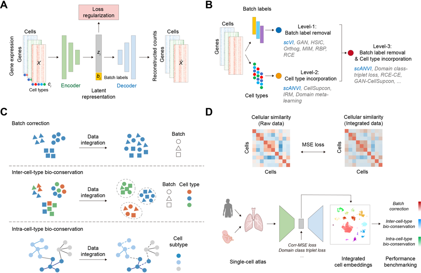
To systematically evaluate various loss functions, we established a unified benchmarking framework wherein all 16 methods were implemented upon a common deep generative model architecture. The framework is built on a conditional variational autoencoder (cVAE) that learns latent representations by conditioning the generative process on variables such as batch labels. The decoder models the count-based nature of scRNA-seq data using a zero-inflated negative binomial (ZINB) distribution.

scVI

The scVI (Single-cell Variational Inference) model [19] served as the foundational baseline for our Level-1 methods. As a probabilistic framework, it generates low-dimensional embeddings suitable for batch correction and other downstream analyses. We selected scVI to benchmark strategies focused exclusively on batch effect removal.

scANVI

The scANVI (Single-cell ANnotation using Variational Inference) model [21], a semi-supervised extension of scVI, was employed as the baseline for Level-2 and Level-3 methods. scANVI incorporates pre-existing cell-type annotations into the generative model to guide the latent space, thereby enhancing the preservation of biological signals during integration. It was selected to evaluate methods that leverage cell-type labels for biological conservation.

Multi-Level loss designs for single-cell data integration

To systematically dissect the impact of information regularization on integration performance, we designed a three-level evaluation framework. Level-1 methods focus on batch effect removal using batch labels; Level-2 methods incorporate cell-type labels for biological conservation; and Level-3 methods utilize both for joint optimization. A total of 16 integration methods were evaluated across these levels.

Level-1: batch effect removal

Methods at this level aim to eliminate batch effects by minimizing the dependence between the latent embeddings and batch labels. The evaluated loss functions include:

GAN

Generative Adversarial Network (GAN) [30] is an adversarial framework that involves a generator and a discriminator engaged in a min-max optimization. The generator creates synthetic samples, while the discriminator distinguishes between real and synthetic ones, with the goal of improving the generator’s ability to produce realistic samples. We adopt the GAN loss design from scGAN [24], tailored for batch effect removal in scRNA-seq data. This loss uses a generator to produce cell embeddings and a discriminator to predict batch labels, generating batch-independent embeddings through adversarial training. The optimization process is described by Eq. (1):

$$\:\underset{\varphi\:}{\text{m}\text{i}\text{n}}\underset{\omega\:}{\text{m}\text{a}x}{\mathbb{E}}_{{q}_{\varphi\:}\left({z}_{ij}|{x}_{ij}\right)}\left[\text{l}\text{o}\text{g}p\left({b}_{j}|{z}_{ij}\right)\right]$$

(1)

where \(\:{x}_{ij}\) represents the scRNA-seq profile of cell \(\:i\) from subject \(\:j\), \(\:{b}_{j}\) is the corresponding batch label, \(\:{z}_{ij}\) is the latent embedding generated by the encoder parameterized by \(\:\varphi\:\), and the discriminator, parameterized by \(\:\omega\:\), predicts \(\:{b}_{j}\) from \(\:{z}_{ij}\).

HSIC

Hilbert-Schmidt Independence Criterion (HSIC) [25] is a non-parametric statistical test that measures the dependence between two random variables using kernel methods. HSIC computes the Hilbert-Schmidt norm of the cross-covariance operator in reproducing kernel Hilbert spaces (RKHS) to quantify the dependence between variables. We minimize the HSIC loss to ensure that cell representations are independent of batch information. The HSIC measure is defined by Eq. (2):

$$\:{\text{H}\text{S}\text{I}\text{C}}_{n}\left(P\right)=\frac{1}{{n}^{2}}\sum\:_{i,j}^{n}\:k({u}_{i},{u}_{j})l({v}_{i},{v}_{j})+\frac{1}{{n}^{4}}\sum\:_{i,j,k,l}^{n}\:k({u}_{i},{u}_{j})l({v}_{k},{v}_{l})-\frac{2}{{n}^{3}}\sum\:_{i,j,k}^{n}\:k({u}_{i},{u}_{j})l({v}_{i},{v}_{k})$$

(2)

where \(\:P\) represents the joint probability distribution of the random variables, the random variable \(\:u\) corresponds to the cell embeddings, and \(\:v\) corresponds to the batch labels, \(\:({u}_{i},{v}_{i})\) are independent and identically distributed (iid) copies of the random variables \(\:u\) and \(\:v\), \(\:k\) and \(\:l\) are kernel functions.

Orthog

Orthogonal Projection Loss (Orthog) is a statistical approach designed to reduce the correlation between two sets of embeddings by applying orthogonal constraints. This loss is minimized to enforce orthogonality between cell embeddings and batch embeddings, effectively disentangling biological signals from technical variations. The loss is formulated as the sum of the squared elements of the covariance matrix:

$$\:{\mathcal{L}}_{\text{O}\text{r}\text{t}\text{h}\text{o}\text{g}}=\:\parallel\:\text{C}\text{o}\text{v}\left({E}_{1},{E}_{2}\right){\parallel\:}_{F}^{2}$$

(3)

where \(\:{E}_{1}\) represents the matrix of cell embeddings and \(\:{E}_{2}\) represents the one-hot encoded matrix of batch embeddings. \(\:\text{C}\text{o}\text{v}\left({E}_{1},{E}_{2}\right)\) denotes the covariance matrix between them.

MIM

Mutual Information Minimization (MIM) is an information-theoretic method that reduces the mutual information (MI) between two variables. MI quantifies the amount of information obtained about one variable through another. To minimize the MI between cell representations \(\:x\) and batch information \(\:y\), we use the definition of MI in Eq. (4):

$$\:\text{I}(x;y)={\mathbb{E}}_{p(x,y)}\left[\text{log}\frac{p(x,y)}{p\left(x\right)p\left(y\right)}\right]$$

(4)

We used the Contrastive Log-ratio Upper Bound (CLUB) [48] estimator to approximate the upper bound of MI by treating it as a divergence between joint and product distributions. To minimize the MI between cell representations and batch information, we apply the sampled vCLUB (vCLUB-S) estimator, which employs a negative sampling strategy to reduce computational complexity. It samples a single negative pair \(\:({\varvec{x}}_{i},{\varvec{y}}_{{k}_{i}^{{\prime\:}}})\) for each positive pair \(\:\left({\varvec{x}}_{i},{\varvec{y}}_{i}\right)\), where \(\:{k}_{i}^{{\prime\:}}\) is uniformly chosen from the set \(\:\{\text{1,2},\dots\:,N\}\), excluding \(\:i\). The MI is then estimated in Eq. (5):

$$\:{\widehat{\text{I}}}_{\text{v}\text{C}\text{L}\text{U}\text{B}-\text{S}}=\frac{1}{N}\sum\:_{i=1}^{N}\:[\text{l}\text{o}\text{g}{q}_{\theta\:}({\varvec{y}}_{i}\left|{\varvec{x}}_{i}\right)-\text{l}\text{o}\text{g}{q}_{\theta\:}\left({\varvec{y}}_{{k}_{i}^{{\prime\:}}}\right|{\varvec{x}}_{i}\left)\right]$$

(5)

where \(\:N\) is the number of samples, and \(\:\theta\:\) represents the parameters of the variational approximation.

RBP

Reverse Backpropagation (RBP) [31] is a domain adaptation method that leverages a Gradient Reversal Layer (GRL) to learn domain-invariant representations. During forward propagation, the GRL functions as an identity transformation. During backpropagation, it reverses the gradient by multiplying it with \(\:-\lambda\:\), where \(\:\lambda\:\) is a fixed meta-parameter:

$$\:{R}_{\lambda\:}\left(\mathbf{x}\right)=\mathbf{x},\:\frac{d{R}_{\lambda\:}}{d\mathbf{x}}=-\lambda\:\mathbf{I}$$

(6)

where \(\:\mathbf{I}\) is the identity matrix. This loss helps eliminate batch-specific signals from the learned representations.

RCE

Reverse Cross-Entropy (RCE) [32] encourages a uniform probability distribution across incorrect classes, introducing ambiguity to enhance the model’s robustness against label noise. We use this loss to distribute labels evenly across batches, reducing batch-specific variations. The RCE loss is defined:

$$\:{\mathcal{L}}_{CE}^{R}(x,y)=-{R}_{y}^{\top}\text{l}\text{o}\text{g}F\left(x\right)$$

(7)

where \(\:x\) is the input feature, \(\:y\) is the target label. \(\:F\left(x\right)\) represents the model output as a probability value or confidence score. \(\:{R}_{y}\:\)is the reverse label vector, where the \(\:y\)-th element is zero, and all others are \(\:\frac{1}{L-1}\), with \(\:L\) as the number of labels.

Level-2: biological information preservation

These methods leverage known cell-type labels to ensure the biological alignment of embeddings across batches. The benchmarked loss functions are:

CellSupcon

Cell Supervised contrastive learning (CellSupcon) applies the principles of supervised contrastive learning [33], leveraging label information to optimize contrastive learning. In this work, cell-type labels are used as class labels, where samples from the same cell type are treated as positives, and those from different cell types are treated as negatives. The CellSupcon loss function incorporates multiple positives and negatives for each anchor sample, eliminating the need for hard negative mining. The loss is defined as:

$$\:{\mathcal{L}}_{\text{out}}^{\text{sup}}=\sum\:_{i\in\:I}\frac{-1}{\left|P\right(i\left)\right|}\sum\:_{p\in\:P\left(i\right)}\text{l}\text{o}\text{g}\frac{\text{exp}({\varvec{z}}_{i}\cdot\:\:{\varvec{z}}_{p}/\tau\:)}{\sum\:_{a\in\:A\left(i\right)}\text{e}\text{x}\text{p}({\varvec{z}}_{i}\cdot\:{\varvec{z}}_{a}/\tau\:)}$$

(8)

where \(\:P\left(i\right)\) represents the set of indices for positive samples, and \(\:A\left(i\right)\) comprises all other indices except \(\:i\). \(\:{\varvec{z}}_{i}\) is the feature vector of the anchor sample, \(\:{\varvec{z}}_{p}\)​ is the feature vector of a positive sample from the same class, and \(\:{\varvec{z}}_{a}\) is the feature vector of any other sample in the mini-batch. The temperature parameter \(\:\tau\:\) is used for normalization.

IRM

Invariant Risk Minimization (IRM) [34] is a method that enhances model generalization by learning features that remain invariant across different environments. It defines a data representation \(\:{\Phi\:}:\mathcal{X}\to\:\mathcal{H}\) that enables an optimal classifier \(\:w:\mathcal{H}\to\:\mathcal{Y}\) to perform consistently across all environments. The goal is to minimize the risk \(\:{R}^{e}\left(\overline{w}\circ\:{\Phi\:}\right)\) for each environment \(\:e\) to ensure stable correlations with the target variable, regardless of environmental variations. IRM is formulated as:

$$\:\underset{{\Phi\:}:\mathcal{X}\to\:\mathcal{Y}}{min}\:\sum\:_{e\in\:{\mathcal{E}}_{\text{t}\text{r}}}\:{R}^{e}\left({\Phi\:}\right)+\lambda\:\cdot\:\parallel\:{\nabla\:}_{w|w=1.0}{R}^{e}(w\cdot\:{\Phi\:}){\parallel\:}^{2}$$

(9)

where \(\:{\mathcal{E}}_{\text{t}\text{r}}\) is the set of training environments, \(\:{\Phi\:}\) is the entire invariant predictor, \(\:w=1.0\) is a fixed “dummy” classifier, and the gradient norm penalty evaluates the classifier’s optimality in each environment. The regularization parameter \(\:\lambda\:\in\:[0,{\infty\:})\) balances predictive power (an empirical risk minimization term) and the invariance of the predictor \(\:1\cdot\:{\Phi\:}\left(x\right)\). We apply IRM by treating batch information as environmental variables and learning invariant features across batches to improve model generalization.

Domain meta-learning

Domain meta-learning [35] is a method designed to improve model adaptability and generalization of models across different domains. It consists of two phases: meta-train and meta-test. In the meta-train phase, the model is trained on labeled data from source domains to learn lower-dimensional representations that effectively predict class labels. This is achieved using a feature extractor defined by \(\:\overline{y}=\sigma\:\left({T}_{\varphi\:}\left({F}_{\theta\:}\left({x}_{i}\right)\right)\right)\), where \(\:{F}_{\theta\:}\left(x\right)\) is the feature extractor for \(\:{x}_{i}\in\:{D}_{t{r}_{i}}\), \(\:{T}_{\varphi\:}\) is a task-specific module, and \(\:\sigma\:\) is the softmax activation. The task-specific loss is defined in Eq. (10):

$$\:{l}_{task}(y,\overline{y};\theta\:,\varphi\:)=-\sum\:_{c}\:1[y=c]\text{l}\text{o}\text{g}\overline{{y}_{c}}$$

(10)

The meta-train phase loss and parameter updates are defined in Eqs. (11 and 12):

$$\:{l}_{meta-train}={l}_{task}\left(y,\overline{y};\theta\:,\varphi\:\right)$$

(11)

$$\:(\theta\:{\prime\:},\varphi\:{\prime\:})=(\theta\:,\varphi\:)-{\alpha\:}_{0}\nabla\:\left[{l}_{meta-train}\right]$$

(12)

In the meta-test phase, the model learns domain-invariant representations to generalize across unseen environments. This involves aligning the geometric configuration of class centroids between domains. The centroid for class \(\:c\) in the domain \(\:d\) is defined as in Eq. (13):

$$\:{\mathcal{C}}_{l,d}^{c}=\frac{1}{{N}_{c}}\sum\:_{({x}_{i},{y}_{i}=c)}\:{F}_{\theta\:}\left({x}_{i}\right)$$

(13)

The alignment loss that measures the difference in pairwise distances between class centroids across meta-train and meta-test domains is defined in Eq. (14):

$$\:{l}_{alignment}(\mathcal{C};\theta\:{\prime\:},\varphi\:{\prime\:})=\sum\:_{c\in\:C}\:\sum\:_{[{d}_{tr},{d}_{ts}]\in\:{D}_{tr}\times\:{D}_{ts}}\:d({\mathcal{C}}_{{d}_{tr}}^{c},{\mathcal{C}}_{{d}_{ts}}^{c})$$

(14)

where \(\:{d}_{tr}\in\:{D}_{tr}\) are the meta-train domains and \(\:{d}_{ts}\in\:{D}_{ts}\) are the meta-test domains. The loss and the parameter update in the meta-test phase are defined in Eqs. (15 and 16):

$$\:{l}_{meta-test}={l}_{task}({d}_{ts};\theta\:{\prime\:},\varphi\:{\prime\:})+\beta\:{l}_{alignment}$$

(15)

$$\:(\theta\:,\varphi\:)=(\theta\:,\varphi\:)-{\alpha\:}_{1}\nabla\:[{l}_{meta-train}+{l}_{meta-test}]$$

(16)

where \(\:{l}_{task}\) is derived from both labeled and unlabeled samples in \(\:{d}_{ts}\),and \(\:\beta\:\) is the regularization coefficient. We use domain meta learning in batch correction to improve the model’s ability to generalize across batches, ensuring consistent features are learned across different batches.

Level-3: joint optimization

Methods at this level jointly optimize for batch-effect removal and biological conservation by integrating both batch and cell-type information. This was achieved by combining loss functions from the previous levels or by using a dedicated loss function:

Domain Class Triplet loss

Domain class triplet loss [36] is an extension of traditional triplet loss designed to integrate domain information for improved generalization across domains. This method modifies the triplet configuration by selecting the positive sample from the same class but a different domain, and the negative sample from the same domain but a different class. The loss function is defined in Eq. (17):

$$\:Los{s}_{DCT}=\left[D\right({a}_{{i}_{c},{i}_{d}},{p}_{{i}_{c},{j}_{d}})-D({a}_{{i}_{c},{i}_{d}},{n}_{{j}_{c},{i}_{d}})+\tau\:{]}_{+}$$

(17)

where \(\:D\) denotes the Euclidean distance, \(\:\tau\:\) is a margin that specifies the separation between the positive and negative pairs. \(\:\alpha\:,p,n\) represent the anchor, positive, and negative samples respectively, with \(\:c\) indicating class labels and \(\:d\) indicating domain labels. We apply this loss to integrate cell type and batch information, optimizing biological signal retention while eliminating batch effects.

scIB-E: an extended framework for evaluating intra-cell-type conservation

For a more holistic evaluation, we developed scIB-E, an extension of the established scIB framework. The scIB-E framework improves upon the original by reorganizing established metrics and, critically, by introducing a novel third category for assessing intra-cell-type biological conservation. The complete framework organizes metrics into the following three distinct categories.

Batch correction metrics

This category is composed of established metrics from the scIB framework that directly quantify the effective removal of batch effects and the mixing of cells from different batches. It includes the following metrics:

Average Silhouette Width (ASW) Batch

Average Silhouette Width (ASW) Batch score quantifies the effectiveness of batch correction by measuring the extent of batch mixing within each cell type. Let batch labels be \(\:{y}_{\text{b}\text{a}\text{t}\text{c}\text{h}}\left(i\right)\in\:\mathcal{B}\). For each cell type \(\:c\in\:\mathcal{C}\), a silhouette score \(\:{s}_{\text{batch}}\left(i\right)\) is computed for each cell \(\:i\) with respect to its batch label, as defined in Eq. (18):

$$\:{s}_{\text{batch}}\left(i\right)=\frac{{b}_{\text{batch}}\left(i\right)-{a}_{\text{batch}}\left(i\right)}{max\left({a}_{\text{batch}}\right(i),{b}_{\text{batch}}(i\left)\right)}\in\:[-\text{1,1}]$$

(18)

where \(\:{a}_{\text{batch}}\left(i\right)\) is the mean distance from cell \(\:i\) to all other cells in the same batch (within cell type \(\:c\)), and \(\:{b}_{\text{batch}}\left(i\right)\) is the mean distance from cell i to all cells in the nearest neighboring batch (within cell type \(\:c\)).

Following common practice, symmetrize and invert so that higher means better mixing:

$$\:{\text{A}\text{S}\text{W}}_{\text{batch}}\left(c\right)=\frac{1}{\left|{C}_{c}\right|}\sum\:_{i\in\:{C}_{c}}(1-|{s}_{\text{batch}}\left(i\right)\left|\right)$$

(19)

The overall batch ASW score is the unweighted mean across cell types,

$$\:{\text{A}\text{S}\text{W}}_{\text{batch}}=\frac{1}{\left|C\right|}\sum\:_{c\in\:C}{\text{A}\text{S}\text{W}}_{\text{batch}}\left(c\right)$$

(20)

where larger values indicate more effective batch integration within each cell type.

Graph Connectivity (GC)

Graph Connectivity (GC) is a batch correction metric that measures the connectivity within label-specific subgraphs in a k-nearest neighbors (kNN) graph. The GC score ranges from 0 to 1, with higher values indicating better batch correction and well-connected cells of the same label, while lower scores suggest poor correction and fragmented subgraphs. The GC score is calculated in Eq. (21):

$$\:\text{G}\text{C}=\frac{1}{\left|C\right|}\sum\:_{\:c\in\:C}\frac{|\text{L}\text{C}\text{C}(G({N}_{c};{E}_{c})\left)\right|}{\left|{N}_{c}\right|}\:$$

(21)

where \(\:C\) denotes the set of cell identity labels, \(\:|\text{L}\text{C}\text{C}(G({N}_{c};{E}_{c})\left)\right|\) is the number of nodes in the largest connected component for each label \(\:c\:\), and \(\:\left|{N}_{c}\right|\) represents the total number of nodes with that label.

Local Inverse Simpson’s Index (iLISI)

Local Inverse Simpson’s Index (iLISI) metric quantifies the degree of batch mixing by measuring the diversity of batch labels within local neighborhoods. Construct a \(\:k\)-nearest-neighbor graph on \(\:\text{X}\). For cell \(\:i\), let \(\:{p}_{\mathcal{l}}\left(i\right)\) be the proportion of neighbors with batch label \(\:\mathcal{l}\in\:\mathcal{B}\) (excluding \(\:i\)). Define the local diversity as in Eq. (22):

$$\:{\text{L}\text{I}\text{S}\text{I}}_{\mathcal{B}}\left(i\right)={\left(\sum\:_{\mathcal{l}\in\:\mathcal{B}}\:{p}_{\mathcal{l}}(i{)}^{2}\right)}^{-1}\in\:[1,|\mathcal{B}\left|\right]$$

(22)

High \(\:{\text{L}\text{I}\text{S}\text{I}}_{\mathcal{B}}\)​ indicates good batch mixing. Rescale per cell to \(\:\frac{{\text{L}\text{I}\text{S}\text{I}}_{\mathcal{B}}\left(i\right)-1}{B-1}\) with \(\:B=\left|\mathcal{B}\right|\), and aggregate by the median as in Eq. (23):

$$\:\text{i}\text{L}\text{I}\text{S}\text{I}=\underset{i}{\text{m}\text{e}\text{d}\text{i}\text{a}\text{n}}\left(\frac{{\text{L}\text{I}\text{S}\text{I}}_{\mathcal{B}}\left(i\right)-1}{B-1}\right)$$

(23)

k-Nearest Neighbor Batch Effect Test (kBET)

kBET (k-nearest neighbor Batch Effect Test) [49] evaluates batch effect correction by comparing local and global batch compositions within a cell’s k-nearest neighbors. The kBET score ranges from 0 to 1, where a higher score means the local batch composition closely matches the global batch composition, indicating better batch effect correction. The kBET score is calculated in Eq. (24):

$$\:\text{k}\text{B}\text{E}\text{T}\text{}=\frac{\sum\:_{i=1}^{N}\mathbb{I}({p}_{i}\ge\:\alpha\:)}{N}$$

(24)

where 𝑁 is the number of neighborhoods, \(\:\mathbb{I}({p}_{i}\ge\:\alpha\:)\)is the indicator function for the \(\:i\)-th neighborhood subset, equal to 1 if the p-value \(\:{p}_{i}\) is greater than or equal to the significance level \(\:\alpha\:\) and 0 otherwise.

Inter-cell-type Bio-conservation metrics

This category also utilizes established label-based metrics from the scIB framework to assess the preservation of biological identity based on discrete cell-type labels. It includes:

Normalized Mutual Information (NMI)

Normalized Mutual Information (NMI) is a statistical metric used to evaluate the similarity between two clustering results. It quantifies the extent of shared information between the two clusterings by normalizing the mutual information (MI) against the geometric mean of their entropies. The NMI score ranges from 0 to 1, where a higher value indicates better agreement between the clusterings, reflecting more accurate correspondence in assignments. The NMI is calculated in Eq. (25):

$$\:\text{N}\text{M}\text{I}=\frac{MI(P,T)}{\sqrt{H\left(P\right)H\left(T\right)}}$$

(25)

where \(\:P\) and \(\:T\) are the two sets of clustering results, \(\:MI(P,T)\) is the mutual information between them, and \(\:H\left(P\right)\) and \(\:H\left(T\right)\) represent the entropies, measuring the randomness within each set of clusters.

Adjusted Rand Index (ARI)

Adjusted Rand Index (ARI) is a metric that measures the similarity between two clustering results. It considers both correct and incorrect assignments, adjusting for chance agreement. The ARI score ranges from 0 to 1, with higher values indicating greater agreement with the ground truth. ARI is calculated in Eq. (26):

$$\:\text{A}\text{R}\text{I}=\frac{TP+TN-E}{TP+TN+FP+FN-E}$$

(26)

where \(\:TP\) and \(\:TN\) are the true positive and true negative pairs, \(\:FP\) and \(\:FN\) are the false positive and false negative pairs, and \(\:E\) is the expected number of random agreements calculated in Eq. (27):

$$\:E=\frac{(TP+FP)\cdot\:(TP+FN)+(FN+TN)\cdot\:(FP+TN)}{TP+TN+FP+FN}$$

(27)

Average Silhouette Width (ASW) Cell Type

Average Silhouette Width (ASW) Cell Type score assesses the preservation of biological structure post-integration by quantifying the separation between distinct cell types in the embedding space. Let the integrated embedding be \(\:X=\{{x}_{i}{\}}_{i=1}^{n}\subset\:{\mathbb{R}}^{d}\) with a distance metric \(\:\varvec{d}(\cdot\:,\cdot\:)\). Denote cell-type labels by \(\:{\varvec{y}}_{\mathbf{c}\mathbf{e}\mathbf{l}\mathbf{l}}\left(\varvec{i}\right)\in\:\mathcal{C}\). Define the silhouette for cell \(\:i\) under the cell-type partition as in Eq. (28):

$$\:{s}_{\text{cell}}\left(i\right)=\frac{{b}_{\text{cell}}\left(i\right)-{a}_{\text{cell}}\left(i\right)}{max\left({a}_{\text{cell}}\right(i),{b}_{\text{cell}}(i\left)\right)}\in\:[-\text{1,1}]$$

(28)

Where \(\:{a}_{\text{cell}}\left(i\right)\) is the mean distance from \(\:{x}_{i}\) to cells sharing \(\:{y}_{\text{cell}}\left(i\right)\), and \(\:{b}_{\text{cell}}\left(i\right)\) is the minimum, over all \(\:{c}^{{\prime\:}}\ne\:{y}_{\text{c}\text{e}\text{l}\text{l}}\left(i\right)\), of the mean distance from \(\:{x}_{i}\) to cells with \(\:{c}^{{\prime\:}}\).

Let \(\:\overline{{s}_{\text{cell}}}=\frac{1}{n}\sum\:_{i=1}^{n}{s}_{\text{cell}}\left(i\right)\). We report the cell-type ASW scaled to \(\:[0,1]\):

$$\:{\text{A}\text{S}\text{W}}_{\text{cell}}=\frac{\overline{{s}_{\text{cell}}}+1}{2}$$

(29)

where larger values indicate better preservation of cell-type structure after integration.

Local Inverse Simpson’s Index (cLISI)

Local Inverse Simpson’s Index (cLISI) metric assesses the preservation of biological structure by measuring the purity of cell-type labels within local neighborhoods. Using the same graph as iLISI, let \(\:{p}_{\mathcal{l}}\left(i\right)\) be the proportion of neighbors with batch label \(\:\mathcal{l}\in\:\mathcal{C}\). Define

$$\:{\text{L}\text{I}\text{S}\text{I}}_{\mathcal{C}}\left(i\right)={\left(\sum\:_{\mathcal{l}\in\:\mathcal{C}}\:{p}_{\mathcal{l}}(i{)}^{2}\right)}^{-1}\in\:[1,|\mathcal{C}\left|\right]$$

(30)

Here, lower diversity signifies well-separated cell types, so we invert and rescale so that higher is better separation as in Eq. (31):

$$\:\text{c}\text{L}\text{I}\text{S}\text{I}=\underset{i}{\text{m}\text{e}\text{d}\text{i}\text{a}\text{n}}\left(\frac{L-{\text{L}\text{I}\text{S}\text{I}}_{\mathcal{C}}\left(i\right)}{L-1}\right)$$

(31)

Isolated label score

Isolated label score is a metric designed to evaluate the effectiveness of data integration in managing cell identity labels that are present in only a few batches. It uses the average silhouette width (ASW) to assess the separation of isolated labels. The score ranges from 0 to 1, with higher values indicating better separation. The isolated label score is defined in Eq. (32):

$$\:\text{Isolated label score}=\frac{1}{N}\sum\:_{i=1}^{N}\left(\frac{1}{{n}_{i}}\sum\:_{j=1}^{{n}_{i}}s\left(j\right)\right)$$

(32)

where \(\:N\) is the number of isolated labels, \(\:{n}_{i}\) is the number of samples in the \(\:i\)-th isolated label, and \(\:s\left(j\right)\) is the silhouette score for each sample \(\:j\).

Intra-cell-type Bio-conservation metrics

This third category is the primary extension introduced in the scIB-E framework, designed to address a key limitation of previous benchmarks by evaluating the preservation of biological variation that is not dependent on cell-type labels. Specifically, we introduced or repurposed the following metrics for this category:

PCR comparison

Principal component regression (PCR) comparison [49] measures the difference in explained variance before and after data integration. The total variance explained by the variable is calculated by summing the variance contributions from its influence across all principal components defined in Eq. (33):

$$\:\text{V}\text{a}\text{r}\left(C|V\right)=\sum\:_{i=1}^{G}\text{V}\text{a}\text{r}\left(C|{\text{P}\text{C}}_{i}\right)\times\:{R}^{2}\left({\text{P}\text{C}}_{i}|V\right)\:\:$$

(33)

where \(\:G\) is the total number of principal components, \(\:C\) denotes the centered data matrix of the dataset under evaluation at a given stage, and \(\:V\) denotes the explanatory variable whose effect is being quantified.\(\:\:\text{V}\text{a}\text{r}\left(C|V\right)\) denotes the total variance in \(\:C\) explained by variable \(\:V\), \(\:\text{V}\text{a}\text{r}\left(C|{\text{P}\text{C}}_{i}\right)\) denotes the variance of \(\:C\) captured by the i-th principal component; and \(\:{R}^{2}\left({\text{P}\text{C}}_{i}|V\right)\) is the squared correlation coefficient indicating how much of the variance of the \(\:i\)-th component is explained by the variable \(\:V\).

The PCR comparison method provides two metrics: PCR comparison-batch and PCR comparison-cell. Both metrics are scaled to a range of 0 to 1, with higher values indicating better performance. In our study, PCR comparison-cell was used to validate the logic of our framework, while PCR comparison-batch was the sole PCR-based metric ultimately incorporated into the scIB-E framework for final performance scoring.

PCR comparison-batch is the PCR-based metric selected for inclusion in the final scIB-E framework. While part of the original scIB benchmark, we have repositioned it to the intra-cell-type conservation category based on its role in our analysis. It serves as a critical proxy to assess over-correction; based on our findings, strong regularization can entangle biological signals with batch effects, and an excessively low score on this metric indicates a corresponding loss of subtle biological signals. The PCR comparison-batch is calculated in Eq. (34):

$$\:\text{P}\text{C}\text{R}\:\text{c}\text{o}\text{m}\text{p}\text{a}\text{r}\text{i}\text{s}\text{o}\text{n}-\text{b}\text{a}\text{t}\text{c}\text{h}=\:\frac{\text{V}\text{a}\text{r}\left({C}_{pre}|B\right)-\text{V}\text{a}\text{r}\left({C}_{post}|B\right)}{\text{V}\text{a}\text{r}\left({C}_{pre}|B\right)}$$

(34)

where \(\:B\) denotes the batch variable, \(\:{C}_{pre}\) and \(\:{C}_{post}\) refer to the original (pre-correction) and integrated (post-correction) data. \(\:\text{V}\text{a}\text{r}\left({C}_{pre}B\right)\) represents the variance in the principal components explained by the batch variable before correction, and \(\:\text{V}\text{a}\text{r}\left({C}_{post}B\right)\) represents the variance in the principal components after correction.

PCR comparison-cell directly quantifies the proportion of cellular variance preserved after integration. Although not incorporated into the final aggregated scIB-E score, it was instrumental in our analysis (e.g., Fig. 3F) for validating that a decrease in the PCR comparison-batch score corresponds to a tangible loss of biological information. The PCR comparison-cell information retention is calculated in Eq. (35):

$$\:\text{P}\text{C}\text{R}\:\text{c}\text{o}\text{m}\text{p}\text{a}\text{r}\text{i}\text{s}\text{o}\text{n}-\text{c}\text{e}\text{l}\text{l}=\:\frac{\text{V}\text{a}\text{r}\left({C}_{pre}|P{C}_{post}\right)-\text{V}\text{a}\text{r}\left({C}_{post}|B\right)}{\text{V}\text{a}\text{r}\left({C}_{pre}|P{C}_{post}\right)}$$

(35)

where \(\:P{C}_{post}\) denotes the set of principal components of the post-correction data. \(\:\text{Var}\left(C_{pre} \mid PC_{post}\right)\:\)represents the variance in the principal components before correction, explained by the principal components after batch correction.

Jaccard index

Jaccard index is a global metric used to evaluate the preservation of cell information during batch correction. It measures the similarity between neighborhood structures by calculating the overlap of k-nearest neighbor graphs between the cell embeddings before and after batch correction. Jaccard index ranges from 0 to 1, with higher values indicating better preservation of neighborhood structures through the batch correction process. The Jaccard index is calculated in Eq. (36):

$$\:\text{Jaccard Index}=\frac{1}{N}\sum\:_{i=1}^{N}\frac{\left|{E}_{{\text{P}\text{C}\text{A}}_{i}}\cap\:{E}_{{\text{e}\text{m}\text{b}\text{e}\text{d}\text{d}\text{i}\text{n}\text{g}}_{i}}\right|}{\left|{E}_{{\text{P}\text{C}\text{A}}_{i}}\cup\:{E}_{{\text{e}\text{m}\text{b}\text{e}\text{d}\text{d}\text{i}\text{n}\text{g}}_{i}}\right|}$$

(36)

where \(\:N\:\)is the number of batches, \(\:{E}_{{\text{P}\text{C}\text{A}}_{i}}\) and \(\:{E}_{{\text{e}\text{m}\text{b}\text{e}\text{d}\text{d}\text{i}\text{n}\text{g}}_{i}}\) represent the sets of edges connecting the k-nearest neighbors in cell embeddings before and after batch correction, respectively.

Corr-MSE: A correlation-based loss for preserving intra-batch structure

To preserve continuous intra-cell-type biological variation independent of discrete cell-type labels, we introduce the Correlation Mean Squared Error (Corr-MSE) loss. This loss function is designed to maintain the global cell correlation structure within each batch during integration.

For each batch, the Pearson correlation coefficient matrices are computed for both the original PCA embeddings and the batch-corrected embeddings. The loss is computed as the mean squared error (MSE) between these two correlation matrices as described in Eq. (37):

$$\:{\mathcal{L}}_{\text{C}\text{o}\text{r}\text{r}-\text{M}\text{S}\text{E}}=\sum\:_{b=1}^{B}\text{M}\text{S}\text{E}\left(\text{C}\text{o}\text{r}\text{r}\left({\mathbf{Z}}_{\text{P}\text{C}\text{A}}^{\left(b\right)}\right),\text{C}\text{o}\text{r}\text{r}\left({\mathbf{Z}}_{\text{c}\text{o}\text{r}\text{r}\text{e}\text{c}\text{t}\text{e}\text{d}}^{\left(b\right)}\right)\right)$$

(37)

where \(\:B\) is the number of batches, \(\:{\mathbf{Z}}_{\text{P}\text{C}\text{A}}^{\left(b\right)}\) represents the original PCA embeddings for batch \(\:b\), and \(\:{\mathbf{Z}}_{\text{c}\text{o}\text{r}\text{r}\text{e}\text{c}\text{t}\text{e}\text{d}}^{\left(b\right)}\) refers to the batch-corrected embeddings for batch \(\:b\).

Benchmarking implementation and evaluationBenchmark datasets and preprocessing

The performance of the benchmarked integration methods was assessed across several diverse, publicly available single-cell RNA-sequencing datasets to ensure the robustness and generalizability of our findings. A consistent preprocessing step was applied to all datasets, where the feature space for analysis was limited to the 4,000 most highly variable genes.

Immune

The immune dataset consists of human immune cells collected from bone marrow and peripheral blood mononuclear cells (PBMCs), sequenced using multiple platforms. It includes 33,506 cells from 10 donors and 16 cell types, collected from five studies. The immune dataset was derived from the study [27].

Pancreas

The pancreas dataset consists of 16,382 cells collected from 9 batches, annotated and classified into 14 distinct cell types. It was obtained from the study [38].

BMMC

The Bone Marrow Mononuclear Cells (BMMC) dataset was created for the 2021 NeurIPS Multimodal Single-Cell Data Integration competition [39]. It contains 90,261 cells and 13,953 genes, originating from bone marrow mononuclear cells collected from multiple donors and sequenced across 12 batches [50]. The dataset includes 45 cell types and is generated using various technologies, such as RNA and protein measurements (CITE-seq) and RNA with chromatin accessibility (10x Multiome). For this analysis, the dataset focuses exclusively on transcriptomic data.

HLCA

The Human Fetal Lung Cell Atlas (HLCA) is an integrated reference atlas of the human respiratory system, including lung parenchyma, respiratory airways, and the nose. We used the core dataset from the HLCA, comprising 584,944 lung cells derived from 166 samples across 107 individuals. The HLCA provides detailed annotations at multiple cell-type levels, along with comprehensive metadata. The dataset was sourced from the study [28].

Human fetal lung cell atlas

The Human fetal lung cell atlas is a dataset based on a multiomic analysis of human fetal lungs, covering 5 to 22 post-conception weeks. This dataset includes 29 batches from 12 donors and spans 8 developmental stages, encompassing 14 broad cell types and 144 newly classified cell types. The dataset was sourced from the study [29].

HBCA

The Human Breast Cell Atlas (HBCA) is a comprehensive single-cell RNA-sequencing dataset of the adult human breast. It comprises over 800,000 cells collected from 55 donors who had undergone reduction mammoplasties or risk-reduction mastectomies, with samples processed across 45 distinct batches. The dataset profiles the three main cellular compartments: epithelial, immune, and stromal, and provides detailed annotations at multiple resolutions, including 11 broad cell types and 41 distinct cell subclusters. The atlas was created to study how cellular composition shifts in response to breast cancer risk factors, including age, parity, and germline BRCA1/2 mutations. The dataset was sourced from the study [41].

Model implementation and hyperparameter optimization

All models were implemented using PyTorch (v1.13.0 + cu117) and trained on a single NVIDIA A100 GPU. Baseline hyperparameters for the scVI and scANVI models were retained from their original implementations (Additional file 2: Table S1). For training, the models were trained for a maximum of 400 epochs, with a batch size of 128. Early stopping was enabled to prevent overfitting.

The various loss functions were integrated into the standard variational autoencoder (VAE) models. The final objective function for each method is a weighted aggregation of the VAE loss (\(\:{L}_{VAE}\)) and the additional regularization loss terms (\(\:{L}_{reg}\)). The general formulation is as follows:

$$\:{L}_{total}=\:{L}_{VAE}+\sum\:_{i=1}^{N}{\lambda\:}_{i}{L}_{reg,i}$$

(38)

where \(\:N\) is the number of regularization terms and\(\:\:{\lambda\:}_{i}\) is the corresponding weight that balances the contribution to the total loss. To systematically determine the optimal weights for each loss function combination, we employed the Ray Tune [37] framework for hyperparameter optimization. The optimization process was conducted on the immune dataset, which was selected as our primary benchmark dataset, with the objective of maximizing the overall scIB total score.

Our parameter selection procedure began by defining a logarithmic search space for each hyperparameter, performing a grid search over the discrete set of values: {0.001, 0.01, 0.1, 1, 10, 100}. For methods in Level-1 and Level-2 involving a single regularization term, we identified the weight that yielded the highest scIB total score. For the CellSupcon loss, while higher weights generally increased the scIB score, our analysis in Fig. 3 revealed that a weight of 10 provided an optimal balance, effectively enhancing biological conservation without significant overcorrection, and was therefore selected for subsequent analyses. For Level-3 methods that combine two regularization loss terms, we simplified the search by fixing the CellSupcon weight at 10 and performing a grid search for the weight of the second loss term. For the RCE-CE method, a two-dimensional grid search was executed. The hyperparameters determined through this optimization process on the immune dataset were then fixed and applied uniformly across all other datasets for the final benchmarking evaluation to ensure a standardized and reproducible comparison. A detailed list of the final hyperparameters used for each of the 16 methods is provided in Additional file 2: Table S2.

Performance score aggregation

The scIB-E framework quantifies overall single-cell integration performance using the scIB-E Total score. This score is a weighted average of the three primary performance categories: batch correction (\(\:{S}_{batch}\)), inter-cell-type biological conservation (\(\:{S}_{inter}\)), and intra-cell-type biological conservation (\(\:{S}_{intra}\)). The aggregation is defined by the formula:

$$\:scIB-{E}_{Total}={w}_{batch}\cdot\:{S}_{batch}+{w}_{inter}\cdot\:{S}_{inter}+{w}_{intra}\cdot\:{S}_{intra}$$

(39)

Each category score (\(\:S\)) is the unweighted arithmetic mean of its constituent metrics (Fig. 4C). The empirically determined weights are set to\(\:\:{w}_{batch}\)=0.2, \(\:{w}_{inter}\)=0.4, and \(\:{w}_{intra}\)=0.4.

These weights were derived from a data-driven optimization procedure designed to ensure that the scIB-E Total score serves as a robust proxy for the preservation of complex biological signals. This procedure utilized the multi-layer annotated Human Lung Cell Atlas (HLCA) dataset. Our objective was to identify a weighting scheme where the scIB-E Total score, calculated using broad level-1 cell annotations for training, maximally correlates with a quantitative benchmark for biological preservation. To establish this benchmark, we first calculated biological conservation scores for each of the finer-grained annotation levels (2, 3, 4, and ‘finest’). The arithmetic mean of these scores served as our final reference, representing a measure of deeper biological truth not exposed to the model.

The optimization involved a grid search over all valid weight combinations, constrained by \(\:{w}_{batch}+{w}_{inter}+{w}_{intra}=1\)and \(\:{0.2\le\:w}_{batch}\le\:0.5\). For each candidate weight combination, we computed the Pearson correlation between the resulting scIB-E Total scores and our quantitative benchmark for biological preservation, assessed across all integration results. The analysis revealed that the weight combination of 0.2 for batch correction, 0.4 for inter-cell-type conservation, and 0.4 for intra-cell-type conservation maximized this correlation. This empirical weighting ensures that the scIB-E Total score is a reliable indicator of an integration method’s ability to balance effective batch removal with the preservation of multi-resolution biological variation.

Downstream task evaluationMoran’s I

Moran’s I is a metric that evaluates the preservation of developmental trajectories in batch-corrected embeddings. It quantifies the global autocorrelation by measuring the correlation between developmental information and graph structures derived from batch-corrected embeddings. Moran’s I ranges from − 1 to 1, with higher values indicating better trajectory preservation. The formula for Moran’s I is defined in Eq. (40):

$$\text{Moran’s } I = \frac{N}{W} \frac{\sum_{i=1}^{N} \sum_{j=1}^{N} w_{ij}(x_i – \bar{x})(x_j – \bar{x})}{\sum_{i=1}^{N} (x_i – \bar{x})^2}$$

(40)

where \(\:N\) denotes the number of cells. \(\:{x}_{i}\) is the developmental information of cell \(\:i\). \(\bar{x}\) is the average developmental information. \(\:{w}_{ij}\) defines neighborhood connectivity, which is 1 if cells are neighbors and 0 otherwise. \(\:W\) is the sum of all connections. For analysis, it is normalized to [0, 1], where values closer to 1 indicate stronger preservation.

Geary’s C

Geary’s C evaluates local differences in developmental information among neighboring cells in batch-corrected embeddings. Its values range from 0 to 2, with lower values indicating better local similarity. The formula for Geary’s C is defined in Eq. (41):

$$\:\text{G}\text{e}\text{a}\text{r}\text{y}{‘}\text{s}\hspace{0.25em}C=\frac{(N-1)}{2W}\frac{\sum\:_{i=1}^{N}\sum\:_{j=1}^{N}{w}_{ij}{\left({x}_{i}-{x}_{j}\right)}^{2}}{\sum\:_{i=1}^{N}{\left({x}_{i}-\bar{x}\right)}^{2}}$$

(41)

where \(\:{w}_{ij}\) is the weight between cells \(\:i\) and \(\:j\), \(\:W=\sum\:_{i,j}{w}_{ij}\:\)is the sum of all weights. For analysis, Geary’s C is normalized to [0, 1], where higher values indicate better preservation of the developmental trajectory.

Differential Abundance (DA) Analysis

We benchmarked the performance of the DCT-Corr method against scVI and scANVI on a differential abundance (DA) analysis task using the Human Breast Cell Atlas (HBCA) [41]. To simulate a realistic workflow, models were trained on 11 broad cell-type labels, while subsequent DA testing was conducted on 41 granular subclusters. We replicated the analytical strategy from the source publication by adopting the Milo [51] methodology. Tests were performed independently within each of the three major cellular compartments (epithelial, stromal, and immune). For each compartment, cell neighborhoods were defined on a k-nearest neighbor (kNN) graph of the integrated embeddings (k = 50, d = 20, prop = 0.3). We then performed four key comparisons using generalized linear models (GLMs) with blocking covariates: (1) the effect of age within the average-risk (AR) cohort (n = 22); (2) the effect of parity within the AR cohort; (3) high-risk BRCA1 mutation carriers (HR-BR1, n = 11) versus the AR cohort; and (4) high-risk BRCA2 mutation carriers (HR-BR2, n = 11) versus the AR cohort. To validate biological discovery, the magnitude of abundance shifts for each subcluster was quantified via the average absolute log-fold change and benchmarked against the findings reported in the source publication [41].