
Our analysis mainly includes three parts: (1) simulation of hydroclimate shock scenarios based on synthetic streamflow data; (2) energy expansion modelling forced by the synthetic streamflow data; and (3) evaluation of climate extreme impacts on energy system development.
Synthetic streamflow generation
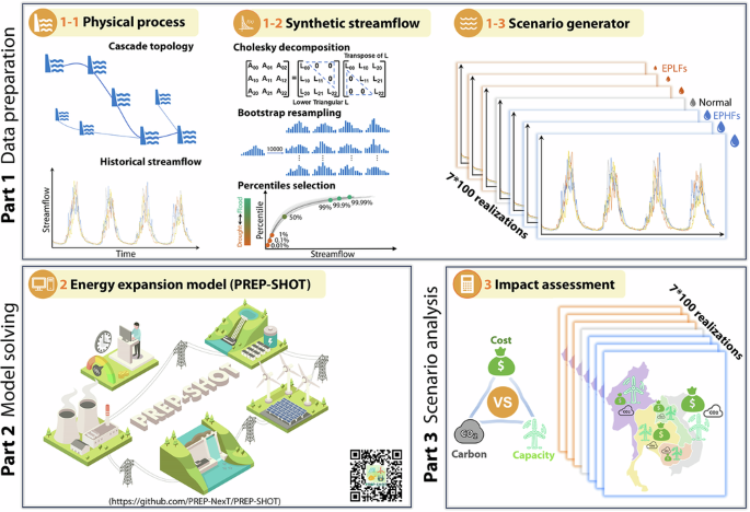
Hydropower development planning in Southeast Asia is limited by a lack of historical hydrometeorological data and an inherent uncertainty of the frequency and intensity of hydroclimate river flow extremes. In the absence of long-term river flow time series, effective planning necessitates the development of synthetic streamflow series that encompass the realm of extreme flows that would ultimately affect hydroelectricity production, a major component of the current renewable energy portfolio in Southeast Asia18,36. Statistical synthetic streamflow generators are cost-effective in simulating a comprehensive range of extreme climate shock scenarios, thereby facilitating robust evaluations of the potential impacts of climate extremes on energy systems64. It should be noted that “climate shock scenarios” refer to synthetic hydroclimatic conditions generated from statistical models based on historical observations in this study. These are distinct from GCM-derived future climate projections and are intended to explore plausible but extreme realizations of baseline climate variability.
Our study employs a non-parametric statistical approach developed by Kirsch et al.65, which not only reproduces key streamflow statistics, such as seasonal means and variances, but also preserves spatial cross-correlations across gauges. Unlike other process-based hydrological models, this generator is driven solely by historical streamflow records without requiring additional data. A number of prior studies have applied this approach to a variety of applications, such as water resources management66 and reservoir operations67.
In our experiments, we generate synthetic streamflow for four representative years (2020, 2030, 2040, and 2050) for 57 existing large hydropower reservoirs within the LMRB (Fig. 2A). This is done under various hydroclimatic scenarios, each including 100 ensemble members. The detailed workflow includes the following 12 steps:
Step 1: Calculate the monthly streamflow data at the outlet of the LMRB by summing the historical daily values.
Step 2: Standardize monthly streamflow values with a log transformation, then reorganize the data into a matrix \(X\) of n rows (years) by 12 columns (months).
Step 3: Compute the cross-month correlation matrix (\(C={X}^{T}\cdot X\)) using standardized historical streamflow data obtained from Step 2. Perform a Cholesky decomposition (\(C=L\cdot {L}^{T}\)), for which L is a real lower triangular matrix with positive diagonal entries and \({L}^{T}\) is its transpose.
Step 4: For each month, bootstrap the standardized streamflow data, recording the associated years as a timestamp to ensure that generated synthetic streamflow time series for other locations maintain the spatial-temporal correlation structure across the entire LMRB domain. Repeat this process 10,000 times to construct a matrix (\({Z}_{0}\)) of random and uncorrelated synthetic streamflow data (10,000 by 12).
Step 5: Impose the temporal autocorrelation structure by multiplying the bootstrapped streamflow \({Z}_{0}\) with the coefficient matrix \(L\) from Step 3: \({Z}_{1}={Z}_{0}\cdot L\), where \({Z}_{1}\) is the resampled standardized streamflow constrained by temporal correlations.
Step 6: Concatenate all \({Z}_{1}\) matrices for all four representative years (2020, 2030, 2040, and 2050).
Step 7: De-standardize the data by applying the inverse log transformation to convert the log-transformed, standardized streamflow values back to their original form. Generate 10,000 realizations of four-year synthetic streamflow data in a matrix format of 10,000 by 48.
Step 8: Rank all 10,000 realizations in ascending order based on their four-year total streamflow. Specifically, EPLF and EPHF scenarios are defined based on the ranking of 10,000 ensemble realizations of four-year cumulative streamflow. These realizations are sorted in ascending order, and specific ranked members are selected to represent different return periods of hydroclimatic extremes. For EPLFs, we select the 1st, 10th, and 100th ranked realizations, corresponding approximately to 1-in-10,000, 1-in-1000, and 1-in-100-year extreme dry conditions, respectively. For EPHFs, we use the 9900th, 9990th, and 10,000th ranked realizations to represent symmetric return periods for extreme wet conditions. Additionally, the 5000th realization, which lies at the median of the distribution, is used to represent a normal hydroclimate scenario.
Steps 1-8 generate synthetic streamflow at the LMRB outlet; however, as we are interested in plant-level hydropower production, we generate synthetic streamflow for each individual upstream reservoir in Steps 9-12.
Step 9: Generate synthetic streamflow into reservoirs, maintaining the spatial-temporal correlation structure of inflows to the 57 reservoirs using the recorded timestamp information of each basin outlet in Step 4 to sample synthetic streamflow. Generate synthetic streamflow data for all reservoirs by selecting their respective historical streamflow data from the same years and months corresponding to the selected extreme and normal scenarios from Step 8.
Step 10: Disaggregate the synthetic monthly streamflow data for all reservoirs into daily data based on their historical observations at daily time scales using the K-Nearest Neighbour (KNN) method68.
Step 11: Repeat Steps 4-10 100 times to construct the ensembles of synthetic streamflow time series.
Step 12: Further disaggregate all daily streamflow data into a four-hourly interval by sampling the daily values repeatedly. This final step prepares the streamflow data for compatibility with the energy capacity expansion model (see details in the next section).
The above steps allow the generation of synthetic streamflow data for four representative years (2020, 2030, 2040, and 2050) and seven climate shock scenarios. These scenarios include one baseline (normal conditions), three wet scenarios (EPHF conditions with return periods of 100, 1000, and 10,000 years), and three dry scenarios (EPLF conditions with return periods of 100, 1000, and 10,000 years). Each scenario comprises 100 ensemble members for 57 selected reservoirs.
Preliminary analysis shows that the synthetic generation algorithm can competently generate streamflow of each individual power plant (Supplementary Table 2). All ensembles of streamflow data generated by the synthetic generation algorithms maintain the same dependencies (spatiotemporal dynamics and cross-correlations among reservoirs on seasonal time scales) and statistical moments as the historical record (see details in Supplementary Fig. 7 and Supplementary Table 2). Coupled with an energy capacity expansion model, this ensemble of synthetic streamflow data enables a quantitative assessment of the impacts of climate extremes on the optimal energy expansion pathways in the LMRB.
Energy capacity expansion model
To identify the optimal energy expansion pathway of LMRB under various climate shock scenarios, we use a modular and open-source energy expansion model: PREP-SHOT4. Compared with other hydropower-centric energy planning models2,5, the unique feature of PREP-SHOT is that it hard-couples a multi-reservoir system model and a power system model. This integration captures two-way feedback between short-term hydropower operation and long-term energy system planning and thereby makes more realistic operational decisions upon the states of both the water and energy systems. This capability is especially critical in regions with a large number of cascade hydropower stations, for example in the LMRB. Details of PREP-SHOT are documented in Liu & He (2023)4. The code of the stable version can be accessed at: https://prep-next.github.io/PREP-SHOT/.
Major inputs of PREP-SHOT include reservoir inflows, existing power infrastructures (such as power plant types, transmission lines, and energy storage; Supplementary Tables 3 and 4), and the capacity factors of VRE. It also incorporates projected electricity load demand over the planning horizon, decarbonization targets, and various techno-economic parameters. These parameters include the lifetime of power technologies and transmission lines, ramping rates for power technologies, lower and upper bounds of the country-level installed capacities of each technology, carbon emission factors of thermal power plants, and electricity transmission topology and efficiency (Supplementary Tables 5 and 6). Additionally, economic factors for each country in the LMRB are considered, including discount rate, investment cost, fixed O&M cost, variable O&M cost, and fuel cost.
All energy technologies included in PREP-SHOT are classified into four categories: (1) ‘hydro’; (2) ‘storage’; (3) ‘non-dispatchable’; and (4) ‘dispatchable’. PREP-SHOT incorporates a ‘hydro’ generation process within specific locations at the plant level. Notably, hydropower in PREP-SHOT not only serves as an important component of electricity generation to meet load demand, but also provides flexibility services to support renewable integration, especially in future energy systems with a high penetration level of VRE. For ‘hydro’, we use synthetic reservoir inflows at four-hour time scales for each modelled year to estimate plant-level hydropower generation. For ‘storage’ technologies, two currently available energy storage technologies, pumped storage hydropower (PSH) and lithium-ion (Li-ion) battery, are considered. PREP-SHOT determines which energy storage type is most cost-effective in facilitating renewable integration, when these energy storage technologies are deployed, and the corresponding capacity of energy storage technologies installed in each country. ‘Non-dispatchable’ technologies consist of solar and wind energy, both of which are limited by capacity factors driven by local weather conditions and installed capacity. ‘Dispatchable’ technologies, including coal-fired plants, oil-fired plants, gas-fired plants and bioenergy, can be controlled within a certain range and usually serve as complementary and flexible power supplies.
Resilient and robust planning of power grids must consider the variably fluctuating energy supply, for example, daily variation of solar and wind energy, intra-annual variability of hydropower generation. This aspect is highly relevant when extreme events are explicitly considered. The energy capacity expansion model must therefore effectively capture the fluctuations in energy supply to ensure that the amount of power generated (electricity supply) is closely balanced with the amount of power being consumed (electricity demand). Traditional models routinely do this by selecting representative days, rather than considering the entire year, to avoid resource-prohibitive computation69. However, this type of short-cut may fail to accurately capture the intra-annual variability of load demand especially when the extreme days of the net load are not included, resulting in an underestimation of the required dispatchable capacity and investment costs when making planning and operational decisions. To avoid this issue, we run four full-year (i.e., representative years 2020, 2030, 2040, and 2050) simulations using PREP-SHOT at four-hourly temporal timesteps (a total of 2,190 = 365*6 time intervals for each modelled year). This solution not only can accurately capture the intra-annual variability of load demand when optimizing the optimal energy expansion pathways but can balance the trade-offs between model representability and computational efficiency. The objective function minimizes the total cost of electricity power planning and operation.
700 synthetic streamflow scenarios (i.e., 100*7 ensembles of four-hourly streamflow time series for each modelled year) are used as inputs for PREP-SHOT to characterize the severities and uncertainties of wetness extremes under different climate shock scenarios. Regarding the spatial resolution, we select five LMRB’s countries as “spatial nodes”: Cambodia, Laos, Thailand, Vietnam, and Myanmar. As the locations of detailed electrical substations in these countries are not publicly available, we model the power transmission lines across different countries as direct connections between the capital of each country (Fig. 2B). Existing and newly installed capacities of all technologies are allocated to each country, as well as future load demand and renewable energy generation time series. Electricity transfer within these five LMRB countries is allowed on the assumption that full coordination can be achieved through the operation of the power grid. The total amount of electricity generation from different energy types and electricity imports (or exports) is restricted to meet the electricity load demand at four-hourly time scales.
PREP-SHOT outputs three major types of variables: water, energy, and cost. Variables related to water systems include the flow released over spillways, as well as storage dynamics for all reservoirs during each time interval. Energy system variables include newly installed capacities during the planning period including different technologies and transmission lines for each modelled year at the country level. These variables are obtained from the cost-optimal pathways using PREP-SHOT. Meanwhile, hourly electricity generation of each technology and transmitted power between paired neighbouring countries per modelled year is also provided to characterize the electricity export or import among each country in LMRB. Cost-related variables include fuel expenses, variable and fixed O&M costs, as well as annualized investment costs for each technology and transmission lines for each modelled year within each country.
Data assumptions and explanationsNatural inflow data
Due to the limited availability of observation-based reservoir inflow data, we use simulated natural inflow obtained from Xu & He (2022)38 to generate synthetic streamflow of all selected reservoirs used in this study (Fig. 2A). Xu and He38 leveraged the calibrated Soil and Water Assessment Tool (SWAT) model to simulate the daily natural inflow of these reservoirs from 1962 to 2005. Furthermore, daily streamflow observations at Kratie station (105.45° E, 12° N, marked in Fig. 2A) over 1962-2005, provided by the MRC, are collected to reflect the regional hydroclimate conditions in LMRB, as it is near to the basin outlet of LMRB (see the section on “Synthetic streamflow generation” for details).
Hydropower generation
Detailed information of plant-level reservoir characteristics and cascade topologies of selected hydropower stations allows capturing realistic hydraulic connections for watersheds with cascade reservoirs. Doing so is essential to accurately simulate the plant-level hydropower generation process especially in regions with a large number of cascade hydropower stations, including some catchments in the LMRB. In this study, we apply a constant water travel time-based routing method to simulate hydraulic delays across cascade systems. This method, commonly used in short-term hydropower operations (Liao et al.)70, effectively captures the timing of water transfers between reservoirs while maintaining computational efficiency in large-scale simulations4. The water travel times used in our model are estimated based on a well-calibrated SWAT model from previous research38, ensuring consistency with the hydrodynamic characteristics of the basin. After translating synthetic streamflow series associated with other relevant system variables to model inputs, PREP-SHOT provides the outputs of hydropower generation at each reservoir at a four-hour resolution, which can characterize the influence of climate extremes on water and energy systems better than aggregating all hydropower generation at country-level with a lower temporal scale. It should be noted that due to institutional restrictions and limited data availability, especially for cross-border or privately operated facilities, we were unable to obtain sufficiently detailed records for validation. Therefore, it is challenging to directly compare simulated hydropower generation against observed data.
Solar and wind energy
We use gridded meteorological variables obtained from Modern-Era Retrospective analysis for Research and Application Version-2 (MERRA-2) reanalysis product71 to estimate the capacity factors of solar and wind power. We select 1986 as the representative year to depict the hourly variations of solar and wind power in each modelled year during 2030-2050, because it can reflect the actual variations of capacity factors in a median year. Furthermore, all hourly values are converted into a four-hourly interval by averaging these data over each four-hourly period with the goal of keeping consistent with the temporal resolution of load demand.
We follow the approach in Liu and He4 to estimate the capacity factors of VRE. For solar power, gridded hourly surface incoming shortwave radiation, top of the atmosphere incoming shortwave radiation, and 2-meter temperature are used to calculate pixel-level capacity factors. The capacity factors of wind energy are calculated using hourly 10- and 50-m wind speeds at each pixel. We aggregate pixel-level capacity factors to country-level by spatially averaging all grid cells within a country, weighted by the pixel area.
In addition to the capacity factors of VRE, we also consider the upper limit of solar energy, which constrains how much solar photovoltaic energy can be produced. This is done by setting different upper bounds in PREP-SHOT for different energy types. The upper bound of solar available in each country of LMRB is based mainly on the approach of Siala et al.72, because the calculation considers topographic and land-use constraints. An Asian Development Bank (ADB) report54 suggests a large potential of wind energy (both onshore and offshore) in LMRB given the vast land and marine areas that are suitable for wind installations. We therefore do not set the technical constraints for wind in PREP-SHOT.
Existing technology capacities and load demand profiles
We collect the 2020 capacity of existing technologies in LMRB, including coal, oil, gas, hydropower, solar, wind, bioenergy, and transmission lines (Fig. 2B) based on published statistics by the Association of Southeast Asian Nations Centre (ASEAN) for Energy73. The capacity and distribution of existing cross-border power transmission lines are acquired from Li & Chang (2015)74. To better depict the load demand profiles in LMRB, we collect country-level hourly electricity data in 2020 from published studies6,19 (see details in Supplementary Note 1). Afterwards, original values are aggregated from hourly to four-hourly intervals to represent the load demand profiles in each modelled year. This aggregation is necessary because it is challenging and computationally expensive to optimize the high-dimensional energy system over an entire year (8,760 h) spanning the full planning horizon that often extends for several decades. In addition, electricity load demand is projected to grow rapidly in the coming decades due to the economic growth in LMRB24. Therefore, we further calculate the four-hourly load demand for each modelled year in the future (2020~2050) by using the projected annual average growth rate of 2.7% for Thailand75, 6.0% for Vietnam76, 8.8% for Cambodia19, 9.5% for Laos19 and 2.7% for Myanmar75 with electricity load demand data in 2020 for each country.
Carbon emission limits
For each modelled year between 2020 and 2050, we collect country-level decarbonization targets from the Climate Action Tracker77, which rates countries based on their efforts to keep temperature increases well below 2 °C and strive for a limit of 1.5 °C above pre-industrial levels. In this study, we use the CAT ratings for the 1.5 °C limit to establish the maximum allowable carbon emissions for each country, ensuring their policies align with the Paris Agreement’s 1.5 °C goal. We then aggregate these carbon emissions across all countries in the LMRB and apply a unified carbon emission constraint that supports the target of limiting long-term warming to 1.5 °C for the entire region.