
Multi-regional input–output model for environmental footprints
Food consumption by households in the EU is strongly related to environmental impacts outside of the EU boundaries through global supply chains and trade networks. Thus, to determine the complete environmental footprints of EU households’ food consumption and their respective changes due to policy-induced consumption changes, we use a multi-regional input–output (MRIO) model. An input–output model represents the interdependence between different economic sectors by quantifying the flow of goods and services between them.
Input–output model
An MRIO model differentiates a standard input–output (IO) model into different regions connected by trade. A standard IO model assumes a single economy of n sectors, each producing total output xi.Matrix A contains technical coefficients aij, which represent the input of sector i required for sector j to produce one unit of output (also referred to as direct requirements). Final demand in each sector i is denoted by yi. Using this notation, the economy can be expressed as
$${\bf{x}}=A{\bf{x}}+{\bf{y}}$$
(1)
This can be reformulated to express total output x in terms of final demand y:
$${\bf{x}}={(I-A)}^{-1}{\bf{y}}$$
(2)
To compute the environmental impacts g induced by final demand y we use the relationship
$${\bf{g}}=S{\bf{x}}=S{(I-A)}^{-1}{\bf{y}}$$
(3)
where S are usage and emission intensities expressed per unit of the economic core.
To differentiate multiple regions, the standard IO model is extended by expanding IO relations to represent the trade between regions. Each region r is represented by a standard IO model, where xr denotes the total output vector, the technical coefficients matrix Ars contains the inputs required by region r from region s, and the final demand vector from region r to region s is denoted by yrs.
Data
We use the global MRIO model EXIOBASE (version 3.8.2)36,37. The model has a well-established history of use in analysing dietary footprints and modelling dietary shift scenarios50. It features global coverage represented by 44 major economies and five rest-of-the-world (RoW) regions. The 27 countries of the EU are represented individually. Furthermore, the model has a detailed and globally consistent sectoral resolution of 200 different product categories. We map the 14 agricultural and ten food-processing sectors onto ten distinct food categories using the concordance table shown in Supplementary Table 2. Of the seven final demand categories included in the model, we only consider final consumption expenditures by households.
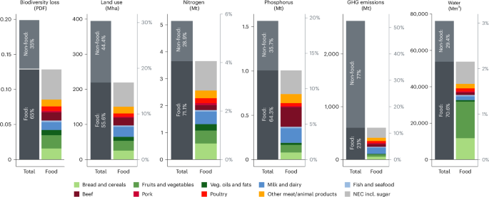
EXIOBASE provides detailed satellite accounts containing 1,113 environmental stressors and 126 impact dimensions. This analysis focuses on GHG emissions, nitrogen and phosphorus emissions, freshwater consumption and land-use stressors (Supplementary Table 3). For phosphorus emissions and freshwater consumption, we directly use characterized impacts as provided by EXIOBASE. In addition, we evaluate 20 available land-use stressors, including 13 cropland, three permanent pasture, two forest area stressors, infrastructure, and total other land use. GHG emissions cover six types of GHG emissions (CO2, methane (CH4), nitrous oxide (N2O), sulfur hexafluoride (SF6), hydrofluorocarbons (HFCs) and perfluorocarbons (PFCs)), which are converted to CO2 equivalents based on most recent estimates of the Global Warming Potential (GWP) 100 metric51. Nitrogen emissions, encompassing emissions to water bodies as well as ammonia (NH3) and nitrogen oxides (NOx) emissions to air, were aggregated into nitrogen impacts using characterization factors provided by EXIOBASE.
We use data for the year 2019. This relies on ‘now-casting’ of the economic structure and all environmental satellite accounts except for CO2 emissions. End years of real data points are 2018 for non-CO2 emissions and 2011 for all other environmental accounts. As a robustness check, results based on real data points only using data for 2011 are shown in Supplementary Figs. 3 and 4 (specification 3, 2011).
Life-cycle impact analysis for biodiversity impacts
To translate the land-use stressors contained in EXIOBASE into spatially explicit impacts in terms of biodiversity loss, we use endpoint characterizations based on LC-IMPACT52. The use of spatially explicit characterization factors recognizes that regionalization has been highlighted as crucial to correctly assessing the impact of land use on biodiversity11. The resulting measure of biodiversity loss reflects an increase in global extinction risk due to land occupation, but does not explicitly consider land transformation, reflecting the time lag between the pressure and its effects as opposed to an immediate global species loss. The LC-IMPACT model uses the global PDF of species as a proxy for biodiversity loss. The global PDF measures the committed global loss of species richness over time as a direct consequence of anthropogenic impacts on ecosystem quality considering individual species’ vulnerability to deteriorating ecosystem quality given that the pressure (here land occupation) persists52. For a single species, a global PDF of 0 reflects no anthropogenic impact, whereas a PDF of 1 corresponds to this species being globally extinct. The global PDF of the LC-IMPACT model is a weighted aggregate of the impact of land use-based stressors on a range of taxonomic groups52. As such, the PDF is an average and not a marginal measure of the impact on biodiversity.
Each of the 20 available land-use stressors from EXIOBASE is assigned to one of six land-use types to translate land occupation into region-specific biodiversity loss (Supplementary Table 3)9,38. The six land-use types are annual crops, permanent crops, pastures, urban, extensive forestry and intensive forestry. We use region-specific characterization factors for 100-year time horizons consistent with the EXIOBASE mapping determined by ref. 38 and made available in an accessible format by ref. 9. Using characterization factors C, biodiversity loss impacts gBL are determined as
$${{\bf{g}}}_{{\rm{BL}}}={C}{{\bf{g}}}_{{\rm{LU}}}$$
(4)
where gLU represents aggregated land-use stressors induced by final demand.
Demand system estimation
Our analysis requires price elasticities to quantify the effect of price increases on the quantities demanded. There are numerous studies estimating price elasticities for various European countries and food categories21,23,24,26,32,53. However, for our purpose, the elasticity estimates in the literature are neither available for all EU27 countries nor consistent with the food categories on which we base our analysis. Thus, we estimate individual demand systems for all EU27 countries to obtain own- and cross-price as well as expenditure elasticities for ten food categories. Specifically, we estimate a linear approximation of the EASI (LA-EASI) implicit Marshallian demand system40.
Linear approximation of the EASI demand system
The EASI demand system is the most recently developed demand system estimation technique, which has substantial advantages over the previously widely used Almost Ideal Demand System (AIDS54) and Quadratic Almost Ideal Demand System (QUAIDS55). In general, the EASI demand system offers a more comprehensive and flexible approach to estimating consumer demand compared to AIDS and QUAIDS. Most importantly, EASI demand systems can estimate nonlinear, flexible Engel curves, which is in line with empirical evidence56. Furthermore, demands are not constrained by Gorman’s rank restriction, error terms can be interpreted as unobserved preference heterogeneity, and, as it is based on expenditure functions, it allows for the derivation of welfare metrics40. We provide a detailed outline of the methodology below and include a summary of all parameter definitions in Supplementary Table 5.
To implement the EASI implicit Marshallian demand system40, we assume that household h with observable characteristics \({{\bf{z}}}_{h}={({z}_{h,\,1},\,\ldots, \,{z}_{h,\,L})}^{{\prime} }\), unobservable preference characteristics \(\bf{{\varepsilon}}_{h}={({\varepsilon }_{h,1},\ldots,{\varepsilon }_{h,n})}^{{{\prime} }}\) with 1nεh = 0 and log nominal total food expenditures xh chooses a bundle of n food categories facing the vector of log prices ph. Thus, following ref. 40, the log food expenditure (or cost) function of household h can be specified as xh = C(ph, uh, zh, εh), expressing the minimum total log expenditures required for household h with characteristics zh and preferences εh to realize utility level uh when facing log prices ph.
Using Shephard’s lemma, the Hicksian budget share functions can be expressed as
$${{\bf{w}}}_{h}={\boldsymbol{\omega }}({{\bf{p}}}_{h},{u}_{h},{{\bf{z}}}_{h},{{\bf{\varepsilon}}}_{h})={{\rm{\nabla }}}_{p}C({{\bf{p}}}_{h},{u}_{h},{{\bf{z}}}_{h},{{\bf{\varepsilon}}}_{h})$$
(5)
where ∇p denotes the vector differential operator evaluated for a change in the price vector p. By replacing indirect utility uh = V(ph, xh, zh, εh) = C−1(ph, ⋅, zh, εh) with the implicit utility yh = g(wh, ph, xh, zh), one obtains the so-called implicit Marshallian demand (or budget share) function
$${{\bf{w}}}_{h}={\boldsymbol{\omega }}({{\bf{p}}}_{h},{y}_{h},{{\bf{z}}}_{h},{{\bf{\varepsilon}}}_{h})$$
(6)
The linear approximation of the EASI demand system assumes that implicit utility yh = g(wh, ph, xh, zh) can be interpreted as the log of real expenditures40, which are log nominal expenditures xh deflated with the Stone price index:
$${y}_{h}={x}_{h}-{{\bf{p}}}_{h}^{{\prime} }{{\bf{w}}}_{h}$$
(7)
We use observed expenditure shares wh to exploit the available household-specific information. We acknowledge that this approach introduces endogeneity, but the linear approximation of the EASI demand system using the Stone price index as defined here has been shown to yield estimates that do not differ substantially from those based on the exact system40. As a robustness check, results using an alternative EASI specification approximating real expenditures using a common Stone price deflator for all households \({\widetilde{y}}_{h}={x}_{h}-{{\bf{p}}}_{h}^{{\prime} }{\bar{{\bf{w}}}}_{h}\) based on the sample mean of expenditure shares, \(\bar{{\bf{w}}}\), are displayed in Supplementary Figs. 3 and 4 (specification 2, ytilda). To reduce numerical problems, yh can be centred in the polynomial regression40. As we did not encounter any numerical problems, our main specification uses the uncentred yh. As a robustness check, results based on yh centred by its sample median, \({y}_{h}^{{\rm{c}}{\rm{e}}{\rm{n}}\mathrm{tr}{\rm{e}}{\rm{d}}}={y}_{h}-\bar{y}\), are displayed in Supplementary Figs. 3 and 4 (specification 4, ycentered).
A convenient estimable functional specification of equation (6) is the following system of equations:
$${{\bf{w}}}_{h}=\underbrace{\mathop{\sum}\limits_{r=0}^{R=4}{\bf{b}}_{r}{y}_{h}^{r}}_{({\rm{I}})}+\underbrace{{A}{\bf{p}}_{h}}_{({\rm{II}})}+\underbrace{{C}{\bf{z}}_{h}}_{({\rm{II}}{\rm{I}})}+\underbrace{{B}{\bf{p}}_{h}{y}_{h}}_{({\rm{IV}})}+\underbrace{{D}{\bf{z}}_{h}{y}_{h}}_{({\rm{V}})}+{{\mathbf{\epsilon}}}_{{h}}$$
(8)
where wh is an n-vector of budget shares that household h spends on the n food categories. The budget share depends on log real total expenditures yh, ph is an n-vector of the food categories’ log prices faced by household h, zh is the L-vector of observable sociodemographics, and b, A, B, C and D are parameter vectors and matrices to be estimated.
The polynomials in term (I) of equation (8) allow for flexible Engel curves, which describe the relationship between budget shares and total expenditures. Term (II) captures the effects of all n prices, and term (III) includes the sociodemographic characteristics that serve as demand shifters, capturing observable heterogeneity between households. The sociodemographics vector zh contains dummy coded information for age (household head is older than 45 years), gender of the household head, presence of children in the household, household income (household income is above median) and urbanity (household is located in a high-population-density area). The terms (IV) and (V) are interaction terms between expenditures and prices, and expenditures and household characteristics, which capture additional heterogeneity in household responses. As a robustness check, results based on equation (8) amended by an additional interaction term \({\sum }_{l=1}^{L}{z}_{h,\,l}{{E}}_{l}{{\bf{p}}}_{h}\) to account for the interaction between household characteristics and prices is shown in Supplementary Figs. 3 and 4 (specification 7, pzintyes).
The model is estimated for each EU27 country individually using sample-weighted seemingly unrelated regression (SUR) to account for the potential correlation of errors across equations within the same household. As a robustness check, results using non-weighted SUR are displayed in Supplementary Figs. 3 and 4 (specification 5, unweighted).
Due to data constraints, we estimate partial demand systems resting on the assumption of weak separability between food and non-food consumption57. In other words, we assume that households first allocate their budget to general consumption categories such as housing, energy, mobility, food and so on. Then, households choose an optimal mix of commodities within each category given their budget constraint for this category (see also refs. 23,32,58). Hence, our demand system estimation only considers food categories and disregards expenditures on other commodities and services. This translates into the assumption that households’ nominal food expenditures remain constant when facing food price changes. As a robustness check, we alternatively estimate incomplete demand systems by including a composite numéraire good that represents all other non-food goods and services consumed by households. Due to a lack of required data for Germany, incomplete demand systems can be estimated for the remaining 26 EU countries only. Results based on the incomplete demand systems thus need to be compared to the partial demand system results excluding Germany in Supplementary Figs. 3 and 4 (specification 6, incomplete; specification 9, partialnoDE).
Adjusting for the censored distribution of budget shares
Due to the restricted duration of recording periods in the household surveys (14 days to 3 months), yearly expenditures for specific food categories may be recorded as zero for some households even though extending the observation period may have resulted in the recording of positive expenditures. Thus, the true expenditure values are only recorded for a subset of all surveyed households. This is a typical sample selection problem where zero observations are the result of an upstream binary choice problem59,60. The resulting censored distribution of the dependent variable of the demand system, the vector of budget shares wh, may result in biased and inconsistent parameter estimates. Therefore, the use of procedures that account for the censored distribution is necessary. As this is not accounted for in the original LA-EASI model specification40, we apply the widely adopted two-step approach for censored distributions of the dependent variable61.
First, we assume a latent variable for the budget share of food category i, \({{w}}_{hi}^{* }\), and a sample selection process that governs which budget shares are observed and which are not:
$$\begin{array}{l}{{w}}_{{hi}}={d}_{{hi}}{{w}}_{{hi}}^{\ast }\,\,\,{\rm{w}}{\rm{i}}{\rm{t}}{\rm{h}}\,\,\,{d}_{{hi}}=\left\{\begin{array}{l}\begin{array}{cc}1 & \mathrm{if}\,{d}_{hi}^{\ast } > 0\end{array}\\ \begin{array}{cc}0 & \mathrm{if}\,{d}_{hi}^{\ast }\le 0\end{array}\end{array}\right.\end{array}$$
(9)
We estimate the probability that the observed budget equals the latent budget share by separately regressing for each food category i a binary outcome variable, di, indicating zero expenditures or not, on a vector of household characteristics sh using probit models:
$${d}_{hi}={{\bf{s}}}_{h}^{{\prime} }{{\boldsymbol{\gamma }}}_{i}+{\zeta }_{hi}$$
(10)
The use of separate probit models implies the assumption of Cov(ζhi, ζhj) = 0 for i ≠ j (ref. 61). Using the estimated vector \({\widehat{{\boldsymbol{\gamma }}}}_{{\boldsymbol{i}}}\), the standard normal cumulative distribution function (cdf) Φ(⋅) and probability density function (pdf) ϕ(⋅) are computed:
$${\widehat{\varPhi }}_{hi}({{\bf{s}}}_{h}^{{\prime} }{\widehat{{\boldsymbol{\gamma }}}}_{i})\,\,\,{\rm{a}}{\rm{n}}{\rm{d}}\,\,\,{\widehat{\phi }}_{hi}({{\bf{s}}}_{h}^{{\prime} }{\widehat{{\boldsymbol{\gamma }}}}_{i})$$
(11)
In the second step, the parameters in equation (8) are estimated correcting for the censored distribution of the observed budget shares (see also ref. 62) with the estimated cdf and pdf values:
$${{\bf{w}}}_{h}={\hat{\Phi}}_{h}\left[\mathop{\sum }\limits_{r=0}^{R=4}{{\bf{b}}}_{r}{y}_{h}^{r}+{{A{\bf{p}}}}_{h}+{{C{\bf{z}}}}_{h}+{{B{\bf{p}}}}_{h}{y}_{h}+{{D{\bf{z}}}}_{h}{y}_{h}\right]+{\hat{\phi}}_{h}{\bf{f}}+{\mathbf{\epsilon}}_{h}$$
(12)
Matrices \({\widehat{\varPhi }}_{h}\) and \({\widehat{\phi }}_{h}\) are n × n identity matrices where the diagonal elements have been replaced by the estimated cdf and pdf values given by equation (11). Homogeneity is satisfied in equation (12) by the use of (log-)normalized prices. That is, we divide all prices by total food expenditures: \({{\bf{p}}}_{h}=\mathrm{ln}(\frac{{\widetilde{{\bf{p}}}}_{h}}{{x}_{h}})\). The symmetry of the Slutsky matrix is ensured by imposing the symmetry of matrices A and B as restrictions in the estimation process. The adding-up restriction does not hold in censoring-corrected demand systems in general, and thus cannot be guaranteed by straightforward parametric restrictions58,63. We therefore use all n equations in the estimation procedure. As a robustness check, results for the uncorrected demand systems, estimated using n − 1 equations and imposing the adding-up restriction, are shown in Supplementary Figs. 3 and 4 (specification 1, uncensored, nmin1).
Prices in the absence of price data
The estimation procedure of the LA-EASI demand system requires the input of prices for each food category included in the demand system. A common problem in demand system estimation is the limited availability of price survey data that can be matched to the household survey data, including food expenditures and quantities62,64. Thus, we use information on quantities purchased per food category available in the household survey data to compute unit values. Unit values are defined as food category expenditure per unit purchased. This is a common approach in the absence of price data. As the products within each food category purchased by each household may vary in quality and price across households, we adjust the unit values65 (see also, for example, refs. 32,66).
Specifically, we regress computed household- and food category-specific unit values UVhi on a vector of household characteristics th. For each of the n food categories, the estimated regression model is given by
$${\rm{UV}}_{{hi}}={\alpha }_{i}+{{\bf{t}}}_{h}^{{\prime} }{\boldsymbol{\beta }}_{i}+{\xi }_{{hi}}$$
(13)
where th contains information on the gender and age of the household head as well as the urbanity of the household location, household size, number of children in the household, and household income (except for Italy where data on household income are missing).
We define the n-vector of adjusted unit value prices as the sum of the regression constant and the predicted residual values:
$${{\bf{p}}}_{h}^{\mathrm{UV}}=\widehat{{\boldsymbol{\alpha }}}+{\widehat{{\boldsymbol{\xi }}}}_{h}$$
(14)
By correcting for quality effects, the adjusted prices proxy the variation in unit values due to supply-side factors. As for households with zero expenditures and where for quantities purchased in a given food category no unit values can be computed, we impute the country median of adjusted unit values. Also, in some countries and for some food categories, the number of households that consumed a specific food category may be relatively low, and we estimate equation (13) only if at least 30 household observations with positive expenditures are available. If fewer than 30 households in country c consumed food category i, no unit value adjustment is conducted, and the non-adjusted unit value is imputed for the adjusted unit value. As a robustness check, results based on non-adjusted unit values are presented in Supplementary Figs. 3 and 4 (specification 8, uvnonadj).
Elasticities
Price elasticities express the percentage change in quantity demanded of food category i due to a 1% price change in food category j (called own-price elasticity for i = j and cross-price elasticity for i ≠ j). The expenditure elasticities express the percentage change in quantity demanded for food category i due to a 1% change in real expenditures y.
From the estimated parameters of equation (12), compensated (Hicksian) elasticities can be computed by dividing Hicksian semi-elasticities by the budget share whi (ref. 40). The Hicksian semi-elasticities with regard to prices are given by
$${\nabla}_{p}^{\prime}{\bf{w}}_{h}={\widehat{\Phi}}_{h}[{A}+{B}{y}_{h}]$$
(15)
and the Hicksian semi-elasticities with regard to real expenditures are
$${\nabla}_{y}{\bf{w}}_{h}={\hat{\Phi}}_{h}\left[\mathop{\sum }\limits_{r=1}^{R=4}r{\bf{b}}_{r}{y}_{h}^{r-1}+{{B{\bf{p}}}}_{h}+{{D{\bf{z}}}}_{h}\right]$$
(16)
Thus, own- and cross-price elasticities are computed using
$${\eta}_{h}^{\mathrm{PE}}={\mathop{\omega}\limits^{\sim}}_{h}^{-1}{\hat{\Phi}}_{h}[{A}+{B}{y}_{h}]+{\mathop{\omega}\limits^{\sim}}_{h}-I$$
(17)
where \({\eta }_{h}^{\mathrm{PE}}\) is an n × n-matrix of compensated price elasticities of household h, \({\widetilde{{\omega }}}_{h}\) is an identity matrix with the ones replaced by the budget shares wh of household h, and I is an n × n identity matrix.
The expenditure elasticities are computed using
$${\boldsymbol{\eta}}_{h}^{\mathrm{EE}}={\mathop{\omega}\limits^{ \sim }}_{h}^{-1}{\hat{\Phi }}_{h}\left[\mathop{\sum }\limits_{r=1}^{R=4}r{{\bf{b}}}_{r}{y}_{h}^{r-1}+{{B{\bf{p}}}}_{h}+{{D{\bf{z}}}}_{h}\right]+{{\bf{1}}}_{n}$$
(18)
where \({{\boldsymbol{\eta }}}_{h}^{\mathrm{EE}}\) is the n × 1-vector of compensated expenditure elasticities of household h.
The compensated elasticities can then be transformed to uncompensated elasticities using the Slutsky equation. Uncompensated (Marshallian) elasticities reflect both substitution and income effects and are used in the policy analysis to compute percentage changes in demanded quantities due to price changes.
Based on the estimated demand system parameters we compute household-specific elasticity estimates. To evaluate country-specific changes in demand due to policy-induced price changes, we compute country-specific weighted-mean elasticities. The household-specific elasticities are weighted by household expenditures and sample weights to ensure the representativeness of the country-specific elasticity estimate with regard to overall expenditures and household composition. The resulting country-specific elasticities are consistent with values found in the literature (Supplementary Table 7) and fall within expected ranges. Supplementary Data 1 provides mean uncompensated own- and cross-price elasticities across EU27 member states (elas) and their standard deviations (s.d.).
Data
To estimate country-specific demand systems of food consumption, we use the Eurostat Household Budget Survey (HBS) for the reference years 2015 and 2010 for 25 out of 27 EU countries. The national household surveys, which are harmonized in the 2015 (2010) HBS data, were conducted by national statistical offices in the years 2014–2016 (2008–2011) and expenditures in euros are adjusted to the respective HBS reference year using price coefficients67. Due to data being missing for Austria and Germany in the HBS dataset, we also use the Konsumerhebung 2014/15 provided by Statistics Austria68, as well as the Einkommens- und Verbrauchsstichprobe (EVS) 2018 provided by the German Federal Statistical Office69. All 27 surveys are representative cross-sectional sample surveys of private households. A common feature is that they collect households’ expenditure information classified along the UN Classification of Individual Consumption by Purpose (COICOP) using diaries maintained over a fixed time period, which varies between countries from two weeks to 3 months67. The data also include selected sociodemographic information of the household and its members (Supplementary Table 4).
For each country covered by the HBS, we consider the most recent available dataset that contains both expenditures and quantities of food items purchased. Specifically, we only use HBS 2010 data if country c has no quantity data for at least one food item available per food category (the aggregation of COICOP level 4 food items into ten food categories is detailed in the following). We remove households that report implausible values on the five-digit (level 4) COICOP classified food items; that is, households are excluded if they report (1) negative expenditures or (2) zero expenditures in combination with positive quantities.
Two cases of missing quantity data have to be considered in the HBS datasets. Case 1 is that the quantities consumed of certain food items i have not been recorded in country c (Supplementary Table 4). Case 2 is that the quantities have been recorded but the recorded data are implausible, as for household h the quantity of food item i is zero and expenditures for food item i are greater than zero. Given the absence of a standardized procedure in the existing literature, we address both cases of missing quantity data separately as outlined in the following.
To address case 1, we use a cross-country matching and imputation algorithm. First, we construct four regions (north, east, south, west) based on the UN geo-scheme for Europe. For each country c, we impute quantities for all food items that have not been recorded. To do so, we construct a matching pool containing all households with positive expenditures from all countries that (1) belong to the same region r as country c and (2) for which quantity data for food item i have been recorded. For each household h of country c that has positive expenditures, the ten nearest neighbours in the matching pool with regard to selected sociodemographic variables, income and expenditures on the specific food item i are found within the matching pool. The missing quantity of food item i for household h in country c is then imputed with the mean of the ten nearest neighbours, weighted by their inverted distance and scaled with the ratio of the distance-weighted-mean expenditures of the ten neighbours and household h’s expenditures. For households with zero expenditures, zero quantities are imputed.
To address case 2, we use a within-country matching and imputation algorithm. For each country c, we impute quantities for all household food item observations that have zero quantities but positive expenditures recorded. To do so, we construct a matching pool containing all households from country c with positive expenditures and positive quantities for food item i. For each household h that has positive expenditures but a zero quantity recorded for food item i, the ten nearest neighbours with regard to selected sociodemographic variables, income and expenditures on the specific food item i are found within the matching pool. The missing quantity for food item i of household h is then imputed with the mean of the ten nearest neighbours, weighted by their inverted distance and scaled with the ratio of the distance-weighted mean expenditures of the ten nearest neighbours and household h’s expenditures.
We aggregate the five-digit (level 4) COICOP classified expenditures on food items into ten distinct food categories (Supplementary Table 2). In addition to the exclusion criteria mentioned above, we exclude (1) households with unreasonably high food expenditures relative to total expenditures (>75%) and (2) households with zero total food expenditures after the matching procedure. Budget shares of different food categories by country are presented in Supplementary Fig. 1. Using the final data on all EU27 countries, we estimate 27 separate LA-EASI demand systems for each country to obtain country-specific elasticity estimates for the ten food categories as described above.
Policy simulation
We simulate two policies inducing different price changes across food categories. For the VAT reform policy, we compute relative price changes of the meat categories using country-specific information on reduced and standard VAT rates (Supplementary Table 1):
$$\frac{\Delta {p}_{c,\,{\rm{m}}{\rm{e}}{\rm{a}}{\rm{t}}}}{{p}_{c,\,{\rm{m}}{\rm{e}}{\rm{a}}{\rm{t}}}}=\frac{1+{r}_{c,\,{\rm{s}}{\rm{t}}{\rm{a}}{\rm{n}}{\rm{d}}{\rm{a}}{\rm{r}}{\rm{d}}}}{1+{r}_{c,\,{\rm{r}}{\rm{e}}{\rm{d}}{\rm{u}}{\rm{c}}{\rm{e}}{\rm{d}}}}-1$$
(19)
where c denotes countries and rc are the VAT rates in country c. This implies that the relative price increase is the same for all meat categories and zero for all non-meat categories.
For the GHG emission price policy, the percentage price increase is determined by country-specific GHG emission intensities and computed as
$$\frac{\Delta {p}_{{ci}}}{{p}_{{ci}}}={\mu }_{{ci}}{\tau }_{{\rm{G}}{\rm{H}}{\rm{G}}}$$
(20)
where μci is the country-specific GHG emission intensity of demand for food category i, displayed in Supplementary Fig. 2. This implies relative price increases for all food categories that vary across categories and countries. The relative price increase, \(\frac{\Delta {p}_{{ci}}}{{p}_{{ci}}}\), only depends on μci as the GHG emission price level, τGHG, isuniform across all food categories and countries. However, as GHG emission intensities are expressed in monetary terms (tCO2e per euro), relative price increases are influenced by the GHG emission content per physical unit of each food category as well as the pre-policy price per physical unit.
The usage of monetary intensities (kgCO2e per euro) is due to the fact that the satellite accounts of EXIOBASE only provide monetary values and no quantities. Just like physical emission intensities (kgCO2e kg−1), monetary emission intensities can be appropriately used for implementing a Pigouvian tax. The monetary emission intensity, μ, of a product can be expressed as
$$\mu =\frac{E/Q}{p}=\frac{E/Q}{X/Q}=\frac{E}{X}$$
(21)
where E are total emissions, Q is physical quantity, p is price per physical quantity and X is total expenditure. This shows that the monetary intensity μ (=E/X) is simply the physical intensity per unit, E/Q, divided by the price per unit, p = X/Q.
When multiplying the monetary intensity by the product price (where τ is the GHG emission price given in euros per tCO2e):
$$\Delta p=\mu \times \tau \times p=\frac{E}{X}\times \tau \times \frac{X}{Q}=\frac{E}{Q}\times \tau$$
(22)
we recover exactly the carbon price applied to physical emissions.
This leads to proper pricing of the externality if the GHG emission price of τ (in € tCO2e−1) ensures that consumers face the full social cost of their consumption choices. For any given product, the tax payment equals monetary intensity times the GHG emission tax times total expenditures:
$$\mu \times \tau \times X=\frac{E}{X}\times \tau \times {pQ}=\frac{E}{X}\times \tau \times \frac{X}{Q}Q=\frac{E}{Q}\times \tau \times Q=E\times \tau$$
(23)
This equals the product’s emissions multiplied by the GHG emission price and thereby adheres to the principle of Pigouvian taxation. The seemingly counterintuitive result presented above that some lower GHG emission intensity food categories face large relative price increases is due to their low pre-policy price per unit. A GHG emission price that will lead to an absolute €1 price increase for products with the same physical emissions per unit will lead to a larger percentage price increase for a €2 product compared to a €20 product. However, although relative price changes may vary, the absolute carbon price signal in € tCO2e−1 remains constant across all food categories and ensures that the externality is priced uniformly across categories.
We assume that the additional cost due to the GHG emission price is not subject to additional VAT. To establish the GHG emission price level (τGHG) necessary to achieve equivalent emission reductions as the VAT reform, the model is iteratively solved.
The vector of percentage changes in the demanded quantities of all food categories in country c depends on both own- and cross-price elasticities:
$$\frac{\Delta {{\bf{q}}}_{c}}{{{\bf{q}}}_{c}}={\eta }_{c}^{\mathrm{PE}}\frac{\Delta {{\bf{p}}}_{c}}{{{\bf{p}}}_{c}}$$
(24)
where \({\eta }_{c}^{\mathrm{PE}}\) is the uncompensated elasticity matrix computed as the country-specific weighted mean from \({\eta }_{{ch}}^{\mathrm{PE}}\) (equation (17)), and \(\frac{\Delta {{\bf{p}}}_{c}}{{{\bf{p}}}_{c}}\) is the vector of relative price changes across all food categories. Thus, the change in footprints associated with consumption of the n food categories in country c is computed as
$$\Delta {{\bf{g}}}_{c}=\frac{\Delta {{\bf{q}}}_{c}}{{{\bf{q}}}_{c}}{{\bf{g}}}_{c}$$
(25)
Welfare analysis
The contrasting policies’ effects on environmental impacts with their corresponding welfare-related costs require a household welfare metric. Given that the EASI demand system is based on an expenditure function model, the estimated parameters of the demand system can be used to compute a closed-form expression of consumer welfare called log cost-of-living (COL)40. As we only capture households’ responses to policy-induced price changes in the demand for food, this welfare metric captures the relative increase in expenditures for food required to sustain the same standard of living with regard to food. Mathematically, it is defined as
$$\begin{array}{rcl}\log ({{\rm{COL}}}_{h}) & = & C({{\bf{p}}}_{h1},{u}_{h0},{{\bf{z}}}_{h},{\bf{\varepsilon}}_{h})-C({{\bf{p}}}_{h0},{u}_{h0},{{\bf{z}}}_{h},{\bf{\varepsilon}}_{h})\\ & = & ({{\bf{p}}}_{h1}-{{\bf{p}}}_{h0}){{\bf{w}}}_{h0}+\frac{1}{2}{({{\bf{p}}}_{h1}-{{\bf{p}}}_{h0})}^{{\prime}}({A}+{B}{{y}}_{h})({{\bf{p}}}_{h1}-{{\bf{p}}}_{h0})\end{array}$$
(26)
where C(⋅) is the log expenditure function. The log COL index is equal to the difference in pre-policy log expenditures, C(ph0, uh0, zh, εh), and log expenditures required to achieve the original level of utility uh0 at post-policy prices ph1. Thus, a positive value corresponds to a welfare loss as households need to expend more to achieve the same level of utility. The index comprises both a first-order effect reflecting a change in purchasing power (given by the Stone index for the price change) and a second-order effect capturing substitution effects between food categories. With major substitution in response to price increases, the latter effect will reduce the overall welfare loss. To obtain absolute monetary values in euros that represent the additional expenditures required to sustain the standard of living with regard to food, we multiply the log(COLh) by households’ total nominal food expenditures, xh:
$$\Delta {\rm{C}}{\rm{O}}{{\rm{L}}}_{h}=\left[({\bf{p}}_{h1}-{\bf{p}}_{h0}){\bf{w}}_{h0}+\frac{1}{2}{({\bf{p}}_{h1}-{\bf{p}}_{h0})}^{\prime}({A}+{{By}}_{h})({\bf{p}}_{h1}-{\bf{p}}_{h0})\right]{x}_{h}$$
(27)
We contrast the additional household expenditures required to sustain the standard of living with regard to food with the additional mean tax income per household generated by the two policies in each country c. For the VAT reform, we determine the change in VAT paid by household h (\(\Delta {T}_{h}^{VAT}\)) as
$$\Delta {T}_{h}^{{\rm{V}}{\rm{A}}{\rm{T}}}=\mathop{\sum }\limits_{i}\left({x}_{hi}^{0}\frac{{r}_{ci}^{0}}{1+{r}_{ci}^{0}}-{x}_{hi}^{1}\frac{{r}_{ci}^{1}}{1+{r}_{ci}^{1}}\right)$$
(28)
where \({x}_{hi}^{0}\) is the observed pre-policy household food expenditures in food category i, \({x}_{hi}^{1}\) is the post-policy household food expenditures, and \({r}_{ci}^{0}\) and \({r}_{ci}^{1}\) are pre- and post-policy VAT rates applied to food category i in country c in which household h resides. Note that for non-meat categories and countries that already apply the standard VAT rate to meat products, \({r}_{ci}^{1}={r}_{ci}^{0}\).
For the GHG emission price policy, we compute the GHG emission price paid by household h (\(\Delta {T}_{h}^{GHG}\)) as
$$\Delta {T}_{h}^{{\rm{G}}{\rm{H}}{\rm{G}}}=\mathop{\sum }\limits_{i}\left({x}_{hi}^{1}\frac{1}{1+{r}_{ci}^{0}}{\mu }_{ci}\,{\tau }^{\mathrm{GHG}}\right)$$
(29)
where μci is the mean GHG emission demand intensity in € tCO2e−1 applied to the net expenditures (\({x}_{hi}^{1}\frac{1}{1+{r}_{ci}^{0}}\)) in food category i for country c in which household h resides and τGHG is the EU-wide GHG emission price level applied. As the GHG emission price policy will also shift demand among the food categories and in some countries different VAT rates are applied to different food categories, we also determine the change in VAT paid by household h for the GHG emission price policy:
$$\Delta {T}_{h}^{{\rm{V}}{\rm{A}}{\rm{T}}}=\mathop{\sum }\limits_{i}\left({x}_{hi}^{0}\frac{{r}_{ci}^{0}}{1+{r}_{ci}^{0}}-{x}_{hi}^{1}\frac{{r}_{ci}^{0}}{1+{r}_{ci}^{0}}\right)$$
(30)
As \({x}_{hi}^{1}\) cannot be observed, we derive the vector of post-policy food expenditures from budget share semi-elasticities:
$${{\bf{x}}}_{h}^{1}=({\bf{1}}+\Delta {{\bf{p}}}^{{\prime} }{{\rm{\nabla }}}_{p}^{{\prime} }{w}_{h}){{\bf{x}}}_{h}^{0}$$
(31)
where \(\Delta {{\bf{p}}}^{{\prime} }\) is the vector of price changes and \({{\rm{\nabla }}}_{p}^{{\prime} }{w}_{h}\) is a matrix of Hicksian price semi-elasticities as given by equation (16). Each element of this matrix gives the change in the budget share wi due to a relative price change in food category j, that is, \(\frac{{\rm{\partial }}{w}_{{hi}}}{{\rm{\partial }}{p}_{{hj}}}\). In the case of the VAT reform, each vector element i of \(\Delta {{\bf{p}}}^{{\prime} }\) is \(\frac{\Delta {p}_{i}}{{p}_{i}}=\frac{1\,+{r}_{i}^{1}}{1+{r}_{i}^{0}}-1\). In the case of the GHG emission price policy, each vector element i of \(\Delta {{\bf{p}}}^{{\prime} }\) is \(\frac{\Delta {p}_{i}}{{p}_{i}}={\mu }_{{ci}}{\tau }_{{\rm{G}}{\rm{H}}{\rm{G}}}\).
Using the household-specific changes in VAT paid and GHG emission price tax revenue we compute EU averages using household and population weights to ensure representativeness.
Monetization of environmental benefits
To allow for an overall evaluation of to what extent the policies increase global aggregate well-being, we monetize the changes in environmental footprints using the global social cost of GHGs, the domestic social cost of nitrogen and the domestic social cost of phosphorus. As the changes in environmental footprints cannot be mapped to the location of impact, we assume that reductions occur proportional to where impacts are generated in the status quo. The social costs represent the welfare-equivalent monetary value of the net damage caused by the emission of an additional unit of the respective substance and thus also represent the net benefit to society resulting from the reduction of emissions by one unit.
The social cost of GHGs encompasses CO2, CH4, N2O, HFCs, PFCs and SF6. We compute the social benefits from reduced GHG emissions using two different sources. First, we refer to ref. 70, which provides social cost estimates for CO2, CH4 and N2O. As specific values for HFCs, PFCs and SF6 are not available in ref. 70, we convert these gases into their CO2 equivalent (CO2e) and apply the social cost of CO2. We also compute the benefits using ref. 71, which provides a substantially higher mean estimate for the social cost of carbon (US$283 versus US$193 per tCO2). As ref. 71 does not provide social cost values for CH4 and N2O, we impute those values using the ratios between their social cost and the social cost of CO2 derived from ref. 70. HFCs, PFCs and SF6 are also converted into CO2e and valued according to the social cost estimate for CO2 in ref. 71. The social cost of nitrogen is quantified based on estimates from ref. 72, which includes the external costs of damage caused by nitrogen leaching and run-off, as well as ammonia (NH3) and nitrogen oxides (NOx) emissions. Both damage to human health and ecosystem impacts are accounted for. The social cost of phosphorus emissions is quantified based on ref. 73, which estimates the external cost of phosphorus emissions into surface waters to be €153.50 per kg. This value is used to compute the local impacts associated with pollution within all EU27 countries. As no robust social cost of nitrogen and phosphorus estimates are available globally, only the value of benefits accruing within the EU is determined. An overview of the social costs assumed is presented in Supplementary Table 6.
Uncertainty quantification
As the MRIO model is provided without associated uncertainty ranges, the only source of uncertainty underlying the policy simulation arises from the estimated elasticities. To quantify the range of uncertainty surrounding our main results, we employ a non-parametric bootstrapping procedure (ref. 74, p. 438), where, for each country c, we treat the original household survey dataset of size Nc as the population and draw b random samples of size Nc with replacement. We set b = 100. Based on each of the b bootstrapping samples, we estimate country-specific demand systems as described in the section ‘Demand system estimation’ to obtain country-specific elasticity estimates. Following the same procedure as described in the section ‘Policy simulation’, we then compute the VAT-equivalent GHG emission price and the footprint reductions for both policy simulations for each of the b obtained country-specific elasticities. This yields b GHG emission price and footprint reduction values. We report the uncertainty as the range between the minimum and maximum of the b computed GHG emission price and footprint reduction values.
Reporting Summary
Further information on research design is available in the Nature Portfolio Reporting Summary linked to this Article.