
EHT datasets on M87*
This work uses the publicly available network-calibrated datasets of M87* (https://eventhorizontelescope.org/for-astronomers/data), reduced through the EHT-HOPS pipeline, on the basis of observations obtained in 2017 (ref. 2), 2018 (ref. 33) and 2021 (ref. 34). In 2017, EHT observations of M87* were conducted with seven separate facilities1: the Atacama Large Millimeter/submillimeter Array (ALMA)49,50, the Atacama Pathfinder Experiment telescope (APEX)51, the Large Millimeter Telescope (LMT)52, the Pico Veleta IRAM 30-m telescope (PV)53, the Submillimeter Telescope Observatory (SMT)54, the James Clerk Maxwell Telescope (JCMT)55 and the Submillimeter Array (SMA)56, which heterogeneously and sparsely sample the Fourier plane as the Earth rotates. Furthermore, the Greenland Telescope (GLT)57,58 participated in the 2018 observations for the first time as part of the EHT array, which improved the aperture coverage, particularly along the north–south direction. For 2021, the 12-m Kitt Peak (KP)59 telescope and the upgraded Northern Extended Millimeter Array (NOEMA)60 facility joined EHT observations for the first time.
The 2017 observations of M87* are spread over four separate epochs (5, 6, 10 and 11 April), whereas observations in 2018 and 2021 are separated into two epochs each (21/25 April for 2018 and 13/18 April for 2021). The datasets with the best single-day aperture coverage each year are 11 April, 21 April and 18 April, which we use as our fiducial datasets, whereas datasets on other days are used as cross-validation. We consider the data taken over two approximately 2-GHz bands centred at 227.1 (low) and 229.1 GHz (high), which we merge into a single dataset.
The interferometric data on M87* comprise complex visibilities, correlated from signals between pairs of stations, referred to as a baseline, which are, by the van Cittert–Zernike theorem61, related to the source brightness distribution by a two-dimensional Fourier transform after certain approximations62. Visibilities can be sequenced into scans, on the basis of the time difference between observations, from which we obtain coherently averaged visibilities. In this work, closure invariants are generally computed from scan-averaged visibilities. With typical scan lengths on the order of five minutes, temporal averaging can potentially introduce residuals from time-dependent gain fluctuations to closure invariants. We have internally validated the robustness of our imaging products by computing closure invariants at the smallest possible cadence of the science-ready dataset (typically 10 s) before scan-level averaging. Following the procedure in the publicly available M87* imaging pipeline (https://github.com/eventhorizontelescope/2019-D01-02), we rescale short baselines to the total flux density estimated from the ALMA and APEX baseline to excise the contribution from extended flux. We have also internally validated that the short baseline rescaling procedure does not affect the recovered morphology from our imaging algorithm. For quantitative comparison, we generate fiducial images from the publicly available eht-imaging pipeline to represent EHTC reconstructions.
Closure invariants
Closure invariants are calibration-independent interferometric measurables produced from a generalized formalism of traditional closure phase24,63 and amplitudes25, with both a co-polar version26 and a polarimetric version27. GenDIReCT uses co-polar closure invariants constructed from elementary triangular plaquette variables called ‘advariants’. The complete minimal set of independent closed triads can be constructed from an array of n stations by selecting all pairs of array elements (a, b) pinned on a fixed reference vertex indexed at 0,
$${{\mathcal{A}}}_{0{ab}}^{{\prime} }={{\mathcal{V}}}_{0a}^{{\prime} }({{\mathcal{V}}}_{{ab}}^{{\prime} \ast }{)}^{-1}{{\mathcal{V}}}_{b0}^{{\prime} }=|{g}_{0}{|}^{2}{{\mathcal{A}}}_{0{ab}},$$
(1)
in which \({{\mathcal{V}}}_{{ab}}^{{\prime} }\) are corrupted visibilities measured from the baseline between stations a and b and |g0|2 is the unknown scaling factor associated with the reference station, which is shared by all complex advariants constructed in this way. By normalizing all advariants by the L2-norm, for example, we produce \({N}_{{\rm{s}}}^{2}-3{N}_{{\rm{s}}}+1\) real-valued independent closure invariants, whose form is different but carry information equivalent to that in traditional closure amplitudes and phases. In the co-polar formalism of closure invariants, traditional closure phases can be identified trivially from the phases of the advariants, whereas closure amplitudes can be derived from specific pairs of advariants. A key advantage of this formalism over traditional closure amplitudes and phases is that it avoids the heterogeneous treatment that phases and amplitudes necessitate. In internal validation tests, closure invariants as the sole likelihood term was found to be preferable over the independently weighted (log-)closure amplitudes and closure phases in terms of convergence and data efficiency.
Various selections of the reference station can affect covariances between closure terms, despite carrying equivalent information. A different selection of reference station can influence the signal-to-noise ratio in the derived closure invariants but does not greatly influence the resulting image reconstruction32. For this work, to avoid bias from a single reference station selection, we present the combined results from two GenDIReCT models for each dataset, trained consistently on the first and the second most sensitive stations as the reference stations in each scan. Selecting from among the most sensitive stations maximizes closure-invariant signal-to-noise ratio and minimizes covariances between closure terms64.
GenDIReCT imaging
The GenDIReCT31 algorithm is an imaging algorithm that uses co-polar closure invariants26 for calibration-independent imaging under the constraints of sparse aperture coverage characteristic of VLBI data. The architecture comprises a latent diffusion model65 conditioned on closure invariants and a multilayer convolutional neural network (CNN) used to optimize the closure invariants likelihood. Traditional imaging algorithms, such as hybrid mapping and self-calibration followed by deconvolution, begin with a simple initial model and iteratively solve for antenna-based complex gains and the image model to converge on a final solution that matches the measured data. These methods can be sensitive to and biased by image initialization and calibration errors, particularly in sparse and low signal-to-noise measurements6,19,22. Our algorithm bypasses the limitations of conventional techniques by using closure invariants as the robust interferometric measurable and produces an image reconstruction directly in a single forward pass. Furthermore, in contrast to the newer regularized maximum likelihood methods that can also image using closure invariants as the sole data term28,35,66,67, our algorithm provides a generative solution that does not require a user-specified, hand-tuned image initialization at inference time. Other machine learning interferometric imaging techniques have been presented in the literature, on the basis of CNNs68,69,70,71,72, normalizing flow73,74, denoising diffusion74,75, classifiers29,76, adversarial networks76,77 and transformers30. Although there are some similarities with other diffusion-based imaging algorithms74,75, GenDIReCT is unique in its closure-conditioned latent diffusion model and, notably, in its use of homogeneous closure invariants rather than the traditional closure phases and closure amplitudes that require heterogeneous treatment. In this section, we provide a brief overview of our algorithm and its past applications.
The neural network architecture is composed of two distinct components. The first component is a conditional U-Net78 based on textually conditioned image generation architectures65 with denoising diffusion probabilistic models79, which has emerged as a highly effective image generation technique, capable of modelling complex data distributions. Our implementation is a latent diffusion model consisting of three convolutional layers set in a symmetric contracting and expanding pathway with residual connections80 from the contracting path that map features to their mirrored expanding layers. In the contracting path, we use one downsampling layer, followed by two downsampling layers with cross-attention, in which the closure-invariant features adjust convolutional features through the cross-attention mechanism, which conditions the denoising process. On the upsampling path, we implement two upsampling layers with self-attention and one final upsampling layer without attention. By having no cross-attention layers in the upsampling path, the result is a robust conditional denoising network that performs well even with noise from real observations. The latent shape is 4 channels of 16 × 16 grids, which is downsampled from the original 64 × 64 total intensity image grid using a pretrained autoencoder30. The second component of the GenDIReCT architecture is a standard multilayer CNN composed of three sequential downsampling layers, designed to compress a large set of diffusion-sampled images (each considered a separate channel) into a representative data-consistent single-channel image reconstruction. We note that we have experimented with several design variations and found this version to be suitable in all tested cases, but better-performing alternatives for specific datasets may be possible.
GenDIReCT works by learning realistic image characteristics (such as positivity and smooth brightness distribution) from a non-astronomical image training dataset, primarily composed of augmented CIFAR-10 natural images81. The conditional latent diffusion model generates sensible image priors, which the multilayer CNN uses as input to optimize the data likelihood and refine the final image reconstruction. As a generative imaging algorithm, our algorithm has the potential to handle degeneracies and visualize multimodalities in the solution space, although they should not be interpreted as image reconstruction uncertainty under a Bayesian framework. Generally, appearance of minor artefacts in low-sensitivity regions, different levels of smoothness and sharpness or super-resolution variations are acceptable consequences of a diversity in potential solutions to the ill-posed image reconstruction problem. However, methodological and hyperparameter sensitivity, or inability to satisfy the underlying measurements, constitute signs that a reconstruction is not robust. By training on unconvolved ground-truth models, GenDIReCT achieves super-resolved reconstructions and enables generative visualization of structural variations that remain strictly consistent with the observed data. Accordingly, unless otherwise indicated, we present unconvolved GenDIReCT outputs optimized to be consistent with the measurements.
We have extensively tested our algorithm on synthetic datasets with the EHT or next-generation EHT (ngEHT) array31, as well as non-horizon-scale EHT datasets on active galactic nuclei, 3C 279 and Centaurus A (ref. 32). On synthetic datasets, our algorithm generalizes well to untrained morphologies and maintains >90% image similarity with ground-truth images at signal-to-noise levels well below the datasets of M87*. Moreover, its performance on quantitative metrics is comparable with other state-of-the-art imaging algorithms on the ngEHT total intensity analysis challenge82. For the EHT dataset on 3C 279, our reconstruction is 98% similar to the EHTC ref. 83, reproducing the core-jet morphology across several independent epochs and enabling direct measurement of the superluminal relative proper motion between components in the image domain. For the EHT dataset on Centaurus A, the EHTC ref. 84 is reproduced with 91% similarity with statistically compatible brightness ratios and opening angle between the north and south edge-brightened jet ridges. These extensive tests on real and synthetic data demonstrate that our algorithm is capable of consistently recovering diverse morphological structures, without manual intervention or prescriptive priors.
Before applying to the real data, each trained model is extensively tested on an array of internal validation tests, which include quantifying its performance degradation with out-of-distribution image morphologies and varying levels of data corruption, accounting for the heterogeneous sensitivity of the array32. Only after passing internal validation are the models unblinded on real data to minimize risk of confirmation bias. No alterations are made to the model between the validation procedure and the unblinding, or post-unblinding.
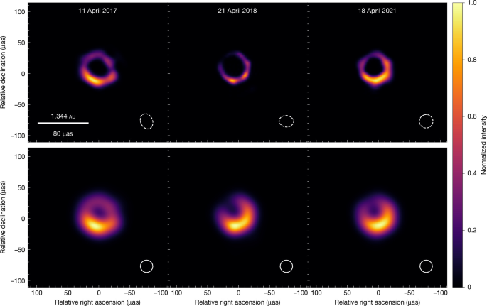
For this work, we train our machine learning architecture with synthetic data derived using the data coverage from all four 2017 and both 2018/2021 observing days independently, combining the two 2-GHz bands into a single scan-averaged dataset for each epoch. We choose 128 × 128-μas2, 225 × 225-μas2 and 450 × 450-μas2 reconstruction fields, each on 64 × 64-pixel grids as predetermined by the architecture. Generally, we represent the aggregate reconstruction for each dataset by the median of all aligned reconstructions. We find the median representation to be more robust against outliers or source alignment issues and a better representation of the bulk of individual image reconstructions. The aggregate reconstructions for all datasets and fields of view are shown in Extended Data Fig. 1 alongside EHTC comparison reconstructions, GenDIReCT composites and a median to median absolute deviation (MAD) ratio panel. The median-to-MAD ratio is presented as a visualization of GenDIReCT’s reconstruction confidence31, in which features of low variance relative to the median pixel intensity (that is, high reconstruction confidence) are highlighted with filled contours.
One of the advantages of the generative imaging process of our algorithm is the potential to explore different imaging solution modes. We consider all observation epochs and all fields of view, presenting the median reconstructions from the most populated solution clusters in Extended Data Fig. 2. Image reconstructions are clustered by Hamming distance in their perceptual hash representation32 to illustrate multimodal solutions. Each cluster is also presented with the best data fidelity score in parentheses. Often, more than 50% of all reconstructions reside within the top two most populous and perceptually similar clusters. This clustering behaviour justifies the pixelwise median as a statistically sound and accurate aggregate representation. The M87* clustering results clearly demonstrate that the differences between reconstruction clusters for the observation days with the highest-quality data are in the surface brightness and extent of extraneous amorphous emission surrounding the ring, rather than fundamental changes to the ring structure itself. For other datasets, solution clusters that are not as clearly ring-like are typically of sparse occurrence in comparison with the bulk of reconstructions and exhibit a lower data fidelity score. On all fields of view, there is no non-ring solution that is favoured over ring-like morphology in the share of the reconstructed image population or data fidelity score. The most ambiguous case is that of the 25 April 2018 dataset, which is missing data from the LMT, resulting in reduced image fidelity compared with the 21 April 2018 observations. The absence of LMT-related baselines created a substantial gap in uv coverage at spatial frequencies corresponding to about 1 Gλ, as the LMT–SMT baseline provided the unique long-baseline constraint for structure in this regime33.
Unless otherwise stated, all models described in this work are trained on augmented non-astronomical images from the CIFAR-10 dataset81, as well as simple geometric shapes, such as Gaussians, disks, rings, ellipses and m-rings85 of the first and second orders31. We present an example grid of augmented training images in Extended Data Fig. 3. Once trained, we run the imaging sequence for 96 total GPU hours on a single NVIDIA H100 GPU for each dataset, producing several hundred (about 300) individual image reconstructions, each drawing from 4,096 diffusion samples. The exact number of final image reconstructions depends on data volume. Although our algorithm has been shown to be generalizable to arbitrary source morphologies31, there is a concern that the presence of crescents and rings in the training dataset may be a source of bias for the image reconstruction. Therefore, we also investigate the outcome of training our architecture without geometric shapes in the training dataset and find no notable difference in the image reconstruction (Extended Data Fig. 3).
Metrics
We use the reduced \({\chi }_{{\rm{CI}}}^{2}\) metric to evaluate the consistency between our image reconstructions with the measurements. The reduced \({\chi }_{{\rm{CI}}}^{2}\) metric is defined as the sum of error-normalized residuals divided by the number of independent data terms,
$${\chi }_{{\rm{CI}}}^{2}=\frac{1}{{N}_{{\rm{ci}}}}\mathop{\sum }\limits_{i}^{{N}_{{\rm{ci}}}}\left[\frac{{({\mathcal{C}}{(A)}_{i}-{C}_{i})}^{2}}{{\sigma }_{i}^{2}}\right],$$
(2)
in which \({\mathcal{C}}\) is an operator that maps the reconstructed image to its closure invariants, indexed by i, for a fixed observation arrangement and Ci is the corresponding closure invariant of the measurement. The total number of closure invariants is denoted by Nci and \({\sigma }_{i}^{2}\) is the estimated uncertainty on the ith closure invariant. We also define the normalized residual of any data point, i, as \(({\mathcal{C}}{(A)}_{i}-{C}_{i})/{\sigma }_{i}\).
Although propagating the estimated uncertainty from each radio station’s system equivalent flux density is straightforward, the total error on each closure invariant is affected by other sources of systematic errors, including time-dependent errors from long coherent visibility averaging and limitations of the linear error propagation model. Generally, the fractional systematic uncertainty budget of 3C 279 and M87 data is about 5%, which is similar in magnitude as measured inter-pipeline differences2. However, in this work, we present our results without further systematic error tolerance and we consistently use as reference the highest-quality single-day EHT-HOPS-reduced pre-scan-averaged dataset of each observation year (11 April for 2017, 21 April for 2018, 18 April for 2021) when evaluating the reduced \({\chi }_{{\rm{CI}}}^{2}\) to ensure a consistent metric across reconstructions. For these datasets, we illustrate the data fidelity from the best GenDIReCT reconstruction and the xsringauss geometric model in Extended Data Fig. 4. A near-unity reduced \({\chi }_{{\rm{CI}}}^{2}\) value confirms that a reconstruction is self-consistent with the measured closure invariants but does not guarantee that the recovered morphology is correct in an absolute sense, making the reduced \({\chi }_{{\rm{CI}}}^{2}\) a necessary but insufficient metric for an accurate reconstruction.
In some cases, it is useful to measure the similarity between reconstructions in the image domain, especially when comparing the GenDIReCT reconstructions with the results from the EHTC imaging pipelines. We measure the image-to-image correspondence with the maximum normalized cross-correlation metric, ρNX, which has the advantage of being independent of image translation and total flux scaling. The metric has been widely used to quantitatively measure image similarity, particularly with image reconstructions produced using only closure data terms28,31,32,82. The ρNX metric is defined as
$${\rho }_{{\rm{NX}}}({I}_{1},{I}_{2})=\frac{1}{M}\text{max}|{{\mathcal{F}}}^{-1}\{{\mathcal{F}}\{\hat{{I}_{1}}\}{\mathcal{F}}{\{\hat{{I}_{2}}\}}^{\ast }\}|,$$
(3)
in which I1 and I2 are two images being compared and the hat operator, \(\hat{I}=(I-\bar{I})/{\sigma }_{I}\), normalizes each image I by its respective flux mean and standard deviation. We denote the forward and inverse Fourier transform as \({\mathcal{F}}\) and \({{\mathcal{F}}}^{-1}\), respectively. The maximum operator ensures that the metric is independent of image translation and it is also useful for aligning separate image reconstructions. To minimize the negative influence of high-frequency artefacts on the maximum normalized cross-correlation, we convolve each image by the fitted clean beam before computing ρNX. Throughout this work, we use ρNX to evaluate the inter-method consistency in resulting image reconstructions, often between the GenDIReCT and EHTC fiducial imaging pipelines or simulated images. As there is no ground-truth reconstruction for M87*, the ρNX metric does not constitute an independent ground-truth validation metric but as an image-domain similarity metric between various imaging algorithms.
Image-domain feature extraction
The image-domain feature extraction method presented here follows the framework established by the EHTC in their initial analysis of M87* (ref. 3). We outline the reproduction of this algorithm below. Given any plausibly ring-like image, we first search for the ring centre, (x0, y0), by evaluating all candidate centroid positions for the one that minimizes the normalized radial peak dispersion
$$({x}_{0},{y}_{0})={\rm{argmin}}\,{\left[\frac{{\sigma }_{r}(x,y)}{{\bar{r}}_{{\rm{pk}}}(x,y)}\right]}_{(x,y)},$$
(4)
in which \({\bar{r}}_{{\rm{pk}}}(x,y)\) is the radius of peak brightness averaged over all angles, as
$${\bar{r}}_{{\rm{pk}}}(x,y)={\langle {{\rm{argmax}}}_{r}[I(r,\theta ;x,y)]\rangle }_{\theta \in [0,2{\rm{\pi }}]},$$
(5)
in which I(r, θ; x, y) is the intensity distribution of the image in radial coordinates, centred on (x, y). The dispersion, σr(x, y), is the corresponding standard deviation of rpk(θ; x, y) across all angles, θ. The ring diameter and its uncertainty can then be identified from \({\bar{r}}_{{\rm{pk}}}(x,y)\) and σr(x, y), respectively, given the measured ring centre, (x0, y0).
Once the ring centre is determined, most other characteristic features can be extracted directly from the polar image, including: the ring width wr, orientation η, azimuthal asymmetry A and central brightness fraction fc. The ring width, wr, is determined by measuring the mean FWHM at each radial slice for the given ring centre,
$${w}_{{\rm{r}}}={\langle {\rm{FWHM}}[I(r,\theta )-{I}_{{\rm{floor}}}]\rangle }_{\theta },$$
(6)
in which the floor value Ifloor = ⟨I(r = 2rpk, θ)⟩θ is used to correct for any non-zero residual flux outside the ring. The uncertainty on the ring width, σw, is measured by the standard deviation in FWHM across all θ.
The orientation angle, η, of the ring (measured east of north) is the circular mean of the first angular mode from rin = rpk − wr/2 to rout = rpk + wr/2, as
$$\eta ={\langle \arg \left[{\int }_{0}^{2{\rm{\pi }}}I(\theta ){{\rm{e}}}^{{\rm{i}}\theta }{\rm{d}}\theta \right]\rangle }_{r\in [{r}_{{\rm{in}}},{r}_{{\rm{out}}}]},$$
(7)
and the corresponding uncertainty, θη, is the standard deviation of the measured angles for r ∈ [rin, rout].
The azimuthal asymmetry, A, is the mean of the normalized amplitude in the first angular mode from rin to rout, which is
$$A={\langle \frac{|{\int }_{0}^{2{\rm{\pi }}}I(\theta ){{\rm{e}}}^{{\rm{i}}\theta }{\rm{d}}\theta |}{{\int }_{0}^{2{\rm{\pi }}}I(\theta ){{\rm{e}}}^{{\rm{i}}\theta }{\rm{d}}\theta }\rangle }_{r\in [{r}_{{\rm{in}}},{r}_{{\rm{out}}}]},$$
(8)
in which σA is the standard deviation in the measured asymmetry over r ∈ [rin, rout]. Perfect azimuthal symmetry corresponds to a value of A = 0, whereas a delta function with all flux concentrated at a single orientation angle corresponds to a value of A = 1.
Finally, the central brightness fraction, fc, is the ratio between the mean interior depression brightness to the mean ring surface brightness, as
$${f}_{{\rm{c}}}=\frac{{\langle I(r,\theta )\rangle }_{\theta ,r\in [0,0.2{r}_{{\rm{pk}}}]}}{{\langle I({r}_{{\rm{pk}}},\theta )\rangle }_{\theta }},$$
(9)
in which the interior brightness is measured from the average flux in a small disk around the ring centre. Although we do not define an uncertainty for a single measurement of fc, we derive its uncertainty from several measurements across the three different fields of view used in GenDIReCT reconstruction. Figure 2 presents the measured ring diameter and orientation across all datasets considered in this work. We present the measurements for ring width, azimuthal asymmetry and central brightness fraction in Extended Data Fig. 5.
The EHTC derived ring parameters using the REX module implemented as part of eht-imaging. Ring properties from three different imaging algorithms (DIFMAP37, eht-imaging28 and SMILI66) were reported for the 2017 data3, two Bayesian imaging algorithms (THEMIS86 and Comrade87,88) were included for the 2018 datasets33 and for 2021 data, one further CLEAN-based algorithm (GPCAL89) and two further regularized maximum likelihood algorithms (DOG-HIT67 and MOEA/D (ref. 35)) were added. However, for the 2021 datasets, the EHTC used an alternative template-matching image-domain feature extraction algorithm34. As such, to maintain methodological consistency, we have reproduced a single eht-imaging reconstruction to use as the EHTC reference.
When comparing ring diameter between datasets, image reconstruction algorithms and across multiyear epochs, there is potential for systematic bias arising from the finite-resolution effect, in which variations in ring width can shift the apparent diameter derived from a direct image-domain feature analysis. Recent EHTC analyses use a forward-modelling procedure to mitigate diameter–width degeneracy34. In this work, we choose to maintain methodological consistency across all reconstructions by deriving diameters directly from the image domain without further adjustment. Therefore, the apparent variation observed between imaging algorithms and individual datasets may be influenced by the finite resolution of each imaging method. Despite this, the apparent ring diameter derived from our reconstructions remains self-consistent across all independent datasets.
Geometric modelling
Our complementary Bayesian analysis uses the geometric xsringauss model4,90, which was designed to simulate the appearance of quasi-Kerr black hole accretion disk radio images91. The advantage of geometric modelling is that visibilities can be derived analytically from simple algebraic expressions and fit to the observed measurements, which substantially reduces the computational requirement of modelling compared with complex and highly nonlinear physical models, particularly when applied with Bayesian sampling algorithms. Moreover, as long as the object is plausibly described by the model, Bayesian sampling methods applied with geometric models enable direct inference of key features of interest from the observed object with associated uncertainties. In this section, we provide a brief description of the xsringauss model, the extra components we included to form the model for fitting and the complete analytical visibility function. We develop the BASIS92 software package for Bayesian analysis with the xsringauss model independent from existing software from the EHTC. For the following discussion, we use \({\mathcal{F}}\) to denote the forward Fourier transform operator.
The xsringauss model is parameterized with the following variables4. The outer disk radius, Rout, and inner disk radius, Rin, create the centralized ‘top-hat crescent’, in which the offset of the inner disk centroid is controlled by the eccentricity, ϵ ∈ [0, 1]. At ϵ = 0, the centres of both disks are co-located at the origin and at the maximum eccentricity, ϵ = 1, the edge of the inner disk meets the edge of the outer disk. The fading parameter, f ∈ [0, 1], controls the surface brightness gradient across the crescent, with the maximum brightness located at the tip of the crescent, at which the crescent width is maximum. When f = 0, the crescent surface brightness is uniform and when f = 1, the surface brightness fades to zero at x = −Rout. Note that we have deliberately adjusted the definition of fading from its original conception90.
The xsringauss model also includes an elliptical Gaussian centred on the inner disk edge, at which the crescent is widest. Its flux is determined by a fraction, fg, of the total flux and its width is set by σe, with axial ratio, ag. The longest axis is always oriented perpendicular to the crescent’s axis of symmetry. A circular Gaussian with flux Vf and width σf centred at x0 represents the floor component internal to the crescent. To complete the base xsringauss model, we blur the image with a circular Gaussian kernel of width σb and rotate the entire image by angle ϕ.
Further components include a larger-scale circular background Gaussian of flux Vbg and width σbg centred at the origin, which is added to include short-spacing flux that is not examined by most of the long-baseline array. Finally, two more nuisance elliptical Gaussians are included, each with independent parameters for flux, width, axial ratio, position angle, angular offsets and Gaussian blur, to capture extraneous amorphous emission that is not modelled by the ring alone and as further degrees of freedom to absorb the effects from measurement errors and systematic uncertainties.
In the Fourier domain, the composite model is a linear combination of elementary components with analytic Fourier transforms. The general Fourier transform (represented by tilde) of a disk with radius R and amplitude V is given by
$$\tilde{D}(\rho )=\frac{{VR}}{\rho }{J}_{1}(2{\rm{\pi }}\rho R),$$
(10)
in which ρ is the Fourier-domain radial coordinate and J1 is a first-order Bessel function of the first kind. The Fourier transform of a Gaussian with flux V and width σ is,
$$\tilde{G}(\rho )=V{{\rm{e}}}^{-2{{\rm{\pi }}}^{2}{\sigma }^{2}{\rho }^{2}},$$
(11)
in which the Fourier transform of asymmetric Gaussians are determined by exploiting the similarity property of the Fourier transform, that is, \({\mathcal{F}}(G({ax},{by}))=\frac{1}{|{ab}|}\tilde{G}\left(\frac{u}{a},\frac{v}{b}\right)\). Multiplication in the image domain of the crescent by the sloped plane is represented in the Fourier domain by taking a derivative
$${\mathcal{F}}(xF(x))=\frac{i}{2{\rm{\pi }}}\frac{{\rm{d}}}{{\rm{d}}s}\tilde{F}(s),$$
(12)
in which, for our specific linear slash function, l(x), the corresponding operation in the Fourier domain is
$${\mathcal{F}}(l(x)F(x))=h\,\left(1-\frac{f}{2}+\frac{i}{2{\rm{\pi }}{R}_{{\rm{out}}}}\frac{f}{2}\frac{{\rm{d}}}{{\rm{d}}s}\right)\tilde{F}(s),$$
(13)
in which the derivatives of Bessel functions of the first kind, Jn, can be expressed in terms of other Bessel functions, Jn±1, as
$$\frac{{\rm{d}}}{{\rm{d}}\rho }{J}_{1}(2{\rm{\pi }}\rho R)={\rm{\pi }}R[\,{J}_{0}(2{\rm{\pi }}\rho R)-{J}_{2}(2{\rm{\pi }}\rho R)],$$
(14)
and h is responsible for normalizing the source to the desired total flux, V, which is dependent on the source structure. For the xsringauss model, the normalization factor is
$$h=\frac{2V}{{\rm{\pi }}\,\left[{R}_{{\rm{out}}}^{2}(2-f)+{R}_{{\rm{in}}}^{2}\left(f\left(1+\frac{{x}_{0}}{{R}_{{\rm{out}}}}\right)-2\right)\right]}.$$
(15)
Each image component can be further independently augmented by translation, rotation and Gaussian blur. In general, image translations are represented with an extra phase term in the Fourier domain, \({{\rm{e}}}^{{\rm{i}}2{\rm{\pi }}({l}_{0}u+{m}_{0}v)}\), in which (l0, m0) denotes the translation in (l, m) coordinates. Image rotation is modelled by a rotation of the uv coordinates. Then, by the convolution theorem, blurring in the image domain with a circular Gaussian kernel is a pointwise multiplication in the Fourier domain by \({{\rm{e}}}^{-{\rm{i}}2{{\rm{\pi }}}^{2}{\sigma }_{{\rm{b}}}^{2}{\rho }^{2}}\), in which σb is the width of the blurring kernel. The final image model and its corresponding analytic Fourier transform is described by 28 parameters. Throughout this work, the xsringauss model is fit to observed data with DYNESTY, a Bayesian dynamic nested sampling algorithm, adopting uniform priors for all parameters. The final fitted image model is formed from the median value of the one-dimensional marginalized posteriors for each parameter. The xsringauss model parameter covariance plot for the highest-quality datasets of 2017 and 2018 is shown in Fig. 3 and we present covariance plots for all other datasets in Extended Data Figs. 6–8. We then apply the image-domain feature extraction analysis on samples from the posterior to measure all characteristic ring parameters (Extended Data Table 1).
Inferring the black hole mass
Inferring the gravitational radius of the black hole from the measured ring diameter requires independently calibrating each imaging method with synthetic data from simulated GRMHD models of lensed black hole accretion emission4. One common simplification is that the observed size of the reconstructed ring should follow a simple scaling relationship with the gravitational radius, dring = αθg. By calibrating to a large ensemble of simulations with different black hole spins, the EHTC determined the calibration factor, α, from the image-domain feature extraction method to be between 10.67 and 11.01, in which the listed range is the result of variations from different image reconstruction algorithms. For geometric modelling methods, the α calibration factor ranges between 11.01 and 12.06. The median of all α calibrations is α ≃ 11.0, which is the calibration factor used by the EHTC for methods that have not been independently calibrated33. Therefore, we also provisionally apply α ≈ 11.0 as our calibration factor in this study.
The associated theoretical uncertainty in the calibrated scaling factor, which arises from recognizing the dataset as a single sample from a dynamic system with unknown physical properties, is σα = 0.4 (ref. 4). In this work, we also use the mean M87* distance measure from the EHTC, which is \(16.{8}_{-0.7}^{+0.8}\,{\rm{Mpc}}\) (ref. 3) based on studies of high-resolution resolved stellar distribution fluctuations13,93 and the tip of the red giant branch standard candle method14.
The prior expectation for the mass of the central black hole in M87 is primarily sourced from high-quality gas12 and stellar11 dynamical estimates, which measured \({M}_{{\rm{gas}}}=3.{5}_{-0.7}^{+0.9}\times 1{0}^{9}{M}_{\odot }\) and Mstar = (6.6 ± 0.4) × 109 M⊙, respectively. The corresponding gravitational radii are \({\theta }_{{\rm{gas}}}=2.{1}_{-0.4}^{+0.5}\,{\rm{\mu }}{\rm{as}}\) and θstar = 3.9 ± 0.3 μas if we use a distance measure of \(16.{8}_{-0.7}^{+0.8}\,{\rm{Mpc}}\). Using the median α = 11.0 ± 0.4 calibration factor and theoretical uncertainty, the prior ring diameters are \({d}_{{\rm{gas}}}=22.{6}_{-4.7}^{+5.9}\,{\rm{\mu }}{\rm{as}}\) and \({d}_{{\rm{star}}}=42.{7}_{-3.6}^{+3.5}\,{\rm{\mu }}{\rm{as}}\). We therefore estimate a black hole mass of \({M}_{{\rm{BH}}}=6.{5}_{-0.4}^{+0.5}\,(11.0/\alpha )\times 1{0}^{9}\,{M}_{\odot }\) with GenDIReCT’s independently measured mean ring diameter. The full range of α = 10.67–12.06 calibration factors implies an estimated black hole mass in the range MBH = (6.0–6.7) × 109 M⊙. On this basis, we conservatively estimate our black hole mass as MBH = (6.5 ± 0.5) × 109 M⊙.
Synthetic M87* images
To compare the reconstructed composites to synthetic M87* images, we retrieve publicly available GRMHD data (https://thz.astro.illinois.edu/resources.html) from the University of Illinois survey41, which includes fluid data for 1,000 time steps (in Rg/c) in the quasi-stationary equilibrium state and five black hole spin prescriptions (a⁎ = −0.94, −0.5, 0, +0.5, +0.94), evolving under the magnetically arrested disk or standard and normal evolution regimes. In this work, we consider only the magnetically arrested disk fluid models, which is the more likely evolutionary scenario for M87* based on jet power constraints94.
Synthetic 230-GHz images of M87* are produced using the general relativistic radiative transfer IPOLE algorithm40 for all time steps, spins and inclination angles between 5° and 90° with a step size of 1°. Note that we use a coupled electron temperature model characterized by Rhigh = 40, which determines the relationship between the ion and electron temperature. Although Rhigh is a free parameter, the time-averaged magnetically arrested disk images are nearly independent of Rhigh and are sensitive primarily on black hole spin for a fixed inclination94. In this work, we compare all beam-convolved synthetic images with the reconstructed M87* composites in the image domain using the normalized cross-correlation metric after correcting for the observer position angle and making linear adjustments to spatial scale, for which both the rotation and scale adjustments of the synthetic images are chosen independently for each parameter combination of spin, inclination and time step, to maximize the resulting normalized cross-correlation comparison with the composite reconstructions. Simulations in ideal GRMHD models are scale-agnostic, enabling such adjustments to be made without affecting the underlying physics41,95. We also repeat our analysis for Rhigh = 80, presenting the figure in the GenDIReCT repository, and find a mild roughly 2° shift towards lower inclinations.