
DataMigration data
We use the IPUMS International dataset, developed and maintained by the University of Minnesota, which consists of census data collected every 5–10 years and harmonized across over 100 countries42. As typical in census exercises, data is collected on a subset of the population – generally, around 10%—that is meant to be representative of the overall population. For each observation, a weight is given by the census institution that illustrates how many actual people this person represents. Note that this dataset does not capture short-term moves, hence we focus on long-term migration patterns. The main benefits of this dataset for our purpose are twofold. First, it provides information on both cross-border and within-country migration. Second, it provides information on demographic characteristics of individuals who have migrated in terms of age, sex, and education. A discussion of its limitations is presented in the Supplementary Discussion. Because mobility patterns vary in nature based on whether the move takes place within a country or across borders, and because the information available for cross-border moves involves a different structure from the one documenting within-country moves (see description below), we treat the two subdatasets separately.
Cross-border migration
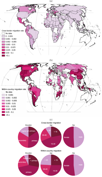
In this part of the dataset, information is gathered at the country level, by the country of destination. We observe the year of migration (1988−2019), as well as the country of residence at time of census (23 countries represented) and the country of birth of the person surveyed (168 countries represented). We assume that a migrant’s country of birth is the country she came from. Cross-border outmigration rates averaged over the period of observations in each country for which weather data is available are shown in Fig. 1a. Average cross-border immigration rates in each destination country for which data is available are shown in Supplementary Fig. S1.
Within-country migration
In this part of the dataset, information is gathered at the level of subnational administrative units (adm1) by the country where the migration is taking place. Information necessary to document within-country migration is available for 71 countries, covering the period 1989−2019. We observe the current location, as well as the prior location defined as location either 1, 5, 10 years ago, or at time of previous census, depending on the country. We use the census data itself to calculate subnational population size, the denominator of our dependent variable. In order to not loose too many observations, we assume that the origin population size at time of migration is the same as its size at time of the last census prior to migration. Finally, as this part of the dataset is less robust than the cross-border migration section, we winsorize the within-country bilateral migration rates to their 0.5-99.5 percentiles. Within-country outmigration rates averaged over the period of observations in each subnational location for which weather data is available are shown in Fig. 1b. We note that migration rates are higher within countries than across borders.
Demographic profiles of migrants
For both within-country and cross-border migration, we calculate migration rates per demographic group for each location and time. Demographics are coded as follows: four categories for education (primary not completed, primary completed, secondary completed, higher education), four categories for age (under 15, 15−30 years old, 30−45, above 45), and two categories for sex (male, female). As we need information on the age, sex, and education of migrants at time of migration, we assume that a migrant’s education at time of migration is the same as her education at time of census. This is a simplifying assumption likely to be false in some cases; yet for the few observations for which a cause of migration is stated, education only represents 6% of cases. We ensure the absence of unrealistic education by forcing lower than secondary education for individuals younger than 15 at time of migration. The distribution of within-country and cross-border migrants over demographic category (education, age, sex) is displayed in Fig. 1c. Cross-border migrants, on average, have higher education levels and are more likely to be of working age than within-country migrants.
In a robustness check, we test the effect of having children at time of migration on the weather-migration relationship (Supplementary Fig. S14). For this additional analysis, the panel unit of analysis is defined not as a function of age, education, and sex, but instead as a function of age, education, and whether the individual had one or more children at time of migration. The latter characteristic is derived from the IPUMS variables giving the age of eldest own child in the household, as well as the year or period of migration.
Population
Our dependent variable is the logged transformation of the outmigration rate, defined as the ratio of number of migrants to population at origin. For cross-border migration, we use data on national level population size. We use the UN World Population Prospects, which provides yearly country-level population for the period 1950−2100. Its historical portion stems largely from census data, and therefore is highly correlated with IPUMS population estimates for available years. Its projection portion is not used here. For within-country migration, we use the census data itself (see subsection “Within-country migration”).
Local temperature data
The Climate Prediction Center compiles and interpolates station measures to produce a gridded daily maximum surface air temperature product with 0. 5∘ by 0. 5∘ resolution from 1979-present43,44. Following51, we use daily maximum rather than mean temperature to better capture human experience of extreme heat stress.
Local soil moisture data
The European Space Agency Climate Change Initiative Plus Soil Moisture Project v06.1 dataset compiles active and passive satellite measures of surface soil moisture down to a depth of 5 cm at daily 0.25∘ × 0.25∘ resolution69,70. Satellite-based measures of surface soil moisture provide a good measure of water availability for plant uptake. See ref. 71 for a detailed discussion, and51,72 for empirical applications to agricultural productivity, a factor relevant to migration. Soil moisture is measured volumetrically, as the volume of water contained within a given volume of soil (i.e., \(\frac{{m}^{3}}{{m}^{3}}\)).
Weighting weather data with population density over the year
For the cross-border migration analysis, we need weather data at the year-by-country level. To that aim, we spatially average the polynomial expansions of daily temperature and soil moisture data over the year across each country, weighting by population density. For the within-country migration analysis, we need weather data at the year-by-subnational unit level. Similarly, we average the polynomial expansions of daily temperature and soil moisture data over the year across each subnational unit. For illustrative purposes, the daily maximum temperature per subnational location for which within-country migration data is available, averaged over the period of observations, is displayed in Supplementary Fig. S3a. A similar representation for soil moisture is displayed in Supplementary Fig. S3b.
Including uncertainty on migration timing in weather data
While the cross-border migration data provides information on the year of migration, the within-country migration data only provides a range of years (see subsection “Within-country migration”). Specifically, 86% of corridor × demographics observations use a specific year, 6% use 1 year periods, 7% use 5 year periods, and 0.5% use 6–10-year periods. In our analysis of within-country movements we use weather levels averaged over the time period corresponding to each census sampling period in order to account for uncertainty in the timing of the migration event. As a robustness check, we use non-averaged weather levels of the earliest possible year of said time period and find similar results for both out-of-sample evaluation and response curves, as makes sense given that observations harboring uncertain migration timing make up less than 8% of the data.
Climate zones
We also explore heterogeneous weather effects on migration across climate zones at origin because the effects of weather variability on mobility are likely to differ depending on the baseline climate. Specifically, we use the Köppen-Geiger climate classification, which identifies five main climate groups and 30 sub-groups52. Here, we consider the five main groups (tropical, dry, temperate, continental, polar), and separate the dry group into two (dry-hot, dry-cold) to better capture effects of temperature and moisture. To map climate zones to the level of our data, we use recent 1 km resolution maps of the Köppen-Geiger climate zones73, and calculate the main climate zone per subnational location or country as the zone associated with the greatest number of people, as computed according to population-weighted grid cells. A geographic representation of the six zones at locations for which migration and weather data is available is given in Supplementary Fig. S3c. We do not present the polar zone in our results because it only accounts for 1% of our observations.
Simulations of temperature and soil moisture under climate change
To project local temperature and soil moisture values under future climate change, we use data from the 6th phase of the Coupled Model Intercomparison Project (CMIP6)74. We extract gridded daily temperature and soil moisture. Temperature is the daily maximum two-meter air temperature (“tmax”) and surface soil moisture is that in the top 10 cm of soil (“mrsos”), which generally accords with satellite measures used in empirical analyses71. We process these to the country-by-year level by first taking polynomial expansions of the daily data and then averaging over the year and national boundaries, weighting by population. We use values from the SSP5-8.5 scenario over two periods: 2015–2035 and 2080–2100. To get a single central estimate we take the median of the processed output over 15 models. The models are ACCESS-ESM1-5, BCC-CSM2-MR, CanESM5, CMCC-ESM2, EC-Earth3, GFDL-CM4, INM-CM4-8, INM-CM5-0, IPSL-CM6A-LR, KACE-1-0-G, MIROC6, MPI-ESM1-2-HR, MPI-ESM1-2-LR, MRI-ESM2-0, and NorESM2-LM.
To estimate local temperature and soil moisture changes for SSP2-4.5 and SSP3-7.0, we apply a pattern scaling approach75. We calculate the SSP2-4.5 and SSP3-7.0 change values by scaling the local changes in temperature and soil moisture from the SSP5-8.5 scenario by the fraction of global mean surface temperature change between the cooler scenario and the warmer scenario. Scaling is performed separately for the linear, quadratic, and cubic weather terms at each location to allow for differential rates of change between average temperature and temperature extremes:
$$\Delta {T}_{i,s} =(\Delta {\bar{T}}_{s}/\Delta {\bar{T}}_{{s}_{o}}) * \Delta {T}_{i,{s}_{o}},\\ \Delta {T}_{i,s}^{2} ={(\Delta {\bar{T}}_{s}/\Delta {\bar{T}}_{{s}_{o}})}^{2} * t \Delta {T}_{i,{s}_{o}}^{2},\\ \Delta {T}_{i,s}^{3} ={(\Delta {\bar{T}}_{s}/\Delta {\bar{T}}_{{s}_{o}})}^{3} * \Delta {T}_{i,{s}_{o}}^{3}$$
(1)
Here s is the scenario of interest, so is the benchmark scenario, i is the location, and \(\bar{T}\) is global mean surface temperature. Scaling for soil moisture is analogous.
We rescale the SSP5-8.5 data rather than using data from SSP2-4.5 and SSP3-7.0 directly because SSP5-8.5 was the scenario for which the largest number of models had available daily temperature and soil moisture projections at the time of analysis, and because the sets of models offering projections differ substantially across scenarios. Using and scaling the SSP5-8.5 projections allows us to incorporate the greatest number of CMIP6 models – 15 – and maintain a constant set of CMIP6 models across various warming levels associated with different SSP scenarios. A large model ensemble enables us to average over and attenuate noise from substantial differences in simulated values across climate models. In addition, maintaining a constant set of climate models across scenarios ensures that differences in results across scenarios are attributable to differences in climatic changes, not to the climate models used. An illustration of how weather variables evolve under medium climate change as represented by the increase in global mean temperature between periods 2015–2035 and 2080–2100 can be found in Supplementary Fig. S16.
Looking at the linear terms, we find that the CMIP6 models yield a local warming that is lower than the global average for 36 countries and higher for 125 countries, which is in line with the fact that land warms more quickly than oceans. We also find that increased global mean temperature leads to dryer conditions in 122 countries, and to wetter conditions in 39 countries, although the cross-model range includes 0 for most countries.
Estimating the effects of weather on migrationEmpirical model
We identify the effect of weather on migration of various demographic groups. The panel unit of analysis is the proportion of people from a specific demographic group (defined as a function of age, education, and sex) that leave their origin to go to a given destination. We compare this unit of observation to itself over time as a non-linear function of temperature and soil moisture of that year in the origin location (Eq. (2)). Note that because mobility patterns vary in nature based on whether the move takes place within a country or across borders, we model within-country migration separately from cross-border migration.
$$\log \left(\frac{mov{e}_{od,t,Z}}{po{p}_{o,t}}\right)= {\beta }_{1}{T}_{o,t}+{\beta }_{2}{T}_{o,t}^{2}+{\beta }_{3}{T}_{o,t}^{3}+{\beta }_{4}S{M}_{o,t}+{\beta }_{5}S{M}_{o,t}^{2} \\ +{\beta }_{6}S{M}_{o,t}^{3}+{\theta }_{od,Z}+{\psi }_{t}+{\delta }_{o}t+{\epsilon }_{od,t,Z}$$
(2)
The migration rate is computed as the ratio of the number of people of demographic characteristics Z moving from origin o to destination d at time t to total population size in o at t. Following22,76, we use the log transformation of the migration rate as the dependent variable. The coefficients of interest are the β coefficients, which give the effects of temperature T and soil moisture SM levels (in degrees Celsius and cm3 of water per cm3 of soil) in cubic form. The cubic form is chosen as the one giving the highest model performance among a linear, quadratic, cubic, or restricted cubic splines model. Similarly, the temperature and soil-moisture pairing gives the highest performance as compared to models using solely temperature, solely soil moisture, solely precipitation, or temperature and precipitation jointly (Supplementary Fig. S17). Vector Z describes demographic characteristics by grouping three indicator variables for the education, age, and sex of migrants.
Time-invariant fixed effects θod,Z are specified for each triplet of origin, destination, and demographic group that account for, e.g., geographic proximity between origin and destination as well as existing diasporas, reflecting the persistence of migration flows. Location-invariant yearly fixed effects ψt are also included to account for migration rate variations that might occur, for example, in response to a global economic shock. Finally, we include a time trend in migration δot for each origin location to account for factors such as technology developments. The residual ϵod,t,Z captures all remaining drivers varying over time within origin-destination-demographic groupings but uncorrelated with the weather variables. We compute standard errors clustering by origin location. Origin locations are subnational for within-country migration and country for cross-border migration.
Testing for heterogeneity across climate zones
As noted earlier, the effects of weather on mobility are likely to differ depending on the baseline climate. To test this hypothesis, we build off Eq. (2), whose terms are indicated by the (2) below.
$$\log \left(\frac{mov{e}_{od,t,Z}}{po{p}_{o,t}}\right)= (2)+{\gamma }_{1}{T}_{o,t}{K}_{o}+{\gamma }_{2}{T}_{o,t}^{2}{K}_{o}+{\gamma }_{3}{T}_{o,t}^{3}{K}_{o}\\ +{\gamma }_{4}S{M}_{o,t}{K}_{o}+{\gamma }_{5}S{M}_{o,t}^{2}{K}_{o}+{\gamma }_{6}S{M}_{o,t}^{3}{K}_{o}$$
(3)
The new terms interact weather variables with an indicator for the climate zone K of the origin location (Eq. (3)).
Testing for heterogeneity across demographic characteristics of migrants
Weather might also affect various demographic groups differently, since observed mobility patterns already differ across demographics. To refine our understanding of who is effected by weather, we interact weather variables in turn with age a, education e, sex s, and their combinations (Eq. (4)).
$$\log \left(\frac{mov{e}_{od,t,Z}}{po{p}_{o,t}}\right)= (2)+{\eta }_{1}{T}_{o,t}{Z}_{i\in \{a| e| s\}}+{\eta }_{2}{T}_{o,t}^{2}{Z}_{i\in \{a| e| s\}}+{\eta }_{3}{T}_{o,t}^{3}{Z}_{i\in \{a| e| s\}}\\ +{\eta }_{4}S{M}_{o,t}{Z}_{i\in \{a| e| s\}}+{\eta }_{5}S{M}_{o,t}^{2}{Z}_{i\in \{a| e| s\}}+{\eta }_{6}S{M}_{o,t}^{3}{Z}_{i\in \{a| e| s\}}$$
(4)
Weather might also affect different demographic groups differently in each climate zone. To test this, we estimate a model building off of models (2)-(4) that additionally interacts weather variables with both demographics and climate zones simultaneously.
Testing for effects of longer-term changes in local climate
As a robustness check we estimate empirical models using temperature and soil moisture values averaged over the 10 years preceding each migration event (Eq. (5)). This approach allows us to examine whether our results, conditioned primarily on single-year weather, alter when examined relative to longer-term changes in local climate. Comparing these effects with effects of shorter-term weather shocks used in our main specifications highlights if and how migration responses change sensitivity over the longer run,
$$\log \left(\frac{mov{e}_{od,t,Z}}{po{p}_{o,t}}\right)= {\nu }_{1}{\sum }_{x=t-9}^{t}\frac{{T}_{o,x}}{10}+{\nu }_{2}{\sum }_{x=t-9}^{t}\frac{{T}_{o,x}^{2}}{10}+{\nu }_{3}{\sum }_{x=t-9}^{t}\frac{{T}_{o,x}^{3}}{10}\\ +{\nu }_{4}{\sum }_{x=t-9}^{t}\frac{S{M}_{o,x}}{10}+{\nu }_{5}{\sum }_{x=t-9}^{t}\frac{S{M}_{o,x}^{2}}{10}+{\nu }_{6}{\sum }_{x=t-9}^{t}\frac{S{M}_{o,x}^{3}}{10}\\ +{\theta }_{od,Z}+{\psi }_{t}+{\delta }_{o}t+{\epsilon }_{od,t,Z}$$
(5)
Assessing the predictive ability of our empirical models
Once the experimental design is set by the fixed effects described in the subsection “Empirical model”, we keep the same design and use the data after removing fixed effects (i.e., the identifying variation) to conduct cross-validation exercises. This process enables us to assess each migration model’s predictive performance out-of-sample. Out-of-sample performance, rather than statistical significance, is used for model selection. To calculate predictive performance, we use 10-fold cross-validation whereby we split the data randomly into 10 folds and use 9 folds for training and the one remaining fold for validation. Models are trained and predictions made for each of the 10 folds. Performance is calculated on these combined out-of-sample predictions using the coefficient of determination (R2), which can be interpreted as the share of variation in migration explained out-of-sample after corridor-by-demographic intercepts, year intercepts and origin-specific trends have been removed. The model R2 considers both errors related to model bias, which stem from the expected value of the estimated function differing from that of the true function, and errors related to model variance, which stem from the estimated function differing from its expected value77. To address potential concerns of over-fitting to the validation set through model selection, we conduct a placebo test where we shuffle the weather observations and refit the model. Consistent with overfitting not being an issue, the shuffled placebo version has no out-of-sample performance across all specifications. To calculate an uncertainty range for the model performance, we use 20 different seeds for splitting the data into 10 folds, and conduct cross-validation for each of the seeds. We present results using the distribution of R2 over the 20 seeds (lower to upper adjacent values). Unless specified otherwise, all hypothesis tests are relative to a null of no effect, and are two-tailed.
To ensure the robustness of our results to the choice of performance metric, we also compute the Continuous Ranked Probability Score (CRPS)78, using the exact same cross-validation procedure (Supplementary Fig. S18). To that aim, we assume a Gaussian distribution of predicted values over the testing sample, and we calculate the CRPS averaged over observations in the testing sample. Note that the CRPS is a measure of the prediction error; a lower CRPS reflects a better performing model. The CRPS gives results that are very similar to those obtained for R2 for both within-country and cross-border migration. For within-country moves, the rankings of model performance based on CRPS and R2 are the same, except that the model including heterogeneity per sex in addition to age and education for each climate zone has a slightly better (lower) CRPS than the model performing best in terms of R2. The Spearman’s rank correlation between R2 and CRPS is -0.98 (note that the negative value results from the opposite ranking order between the two metrics). For cross-border migration, model ranking remains similar across R2 and CRPS performance metrics, except that the model allowing differences per climate zone interacted with age and education gives the best (lowest) CRPS score, on average, though with a much more variable score. The Spearman’s rank correlation between R2 and CRPS is -0.39 if including this model, and -.81 if not. Given this model’s low and uncertain predictive performance as measured by the R2, and its uncertain performance as expressed by the CRPS, we instead choose the model allowing for differences per age, education, and climate zone as our primary specification because it performs best in terms of R2 and second best in terms of CRPS. Overall, we use the best model according to R2, because of its simplicity of interpretation (variance explained) and common use in the literature, and note that findings are generally consistent with model selection based on CRPS.
We perform cross-validation for our main line of results by splitting data into random folds in order to evaluate the ability of models to explain historical migration. To more fully characterize how our best performing models can be used for prediction in policy-relevant contexts, we conduct additional tests of model ability to temporally extrapolate by splitting the data into folds by year, as opposed to the random splits as done in the main analysis. This approach forces predictions to be made and evaluated for years not represented in the training data and is of specific use for evaluating model use in future climate change projections.
For both within-country and cross-border migration, our best performing models maintain positive performance over time, though their performance is not significantly different from zero (Supplementary Fig. S8). To account for the additional challenge of extrapolating over time, we try a simpler model for cross-border migration, whereby we restrict the dimensions of heterogeneity considered to age and education, and use a linear rather than cubic functional form for temperature, as temperature responses are found to be approximately linear (Fig. 2b). We find that this simpler model generalizes better to held-out observations over time (out-of-sample R2 = 0.0010 [0.0005;0.0015]) and thus use it for climate change projections. A representation of its response curves is given in Supplementary Fig. S9.
Projections in a future with increasing climate change
Once the best performing model is selected, we use it as basis for a projection exercise of migration patterns with increasing climate change over the 21st century. As a straightforward application, we project this model assuming that climate is the only changing factor while other drivers of migration do not otherwise change. To project local temperature and soil moisture values under future climate change, we use data from the 6th phase of the Coupled Model Inter-comparison Project (CMIP6). We extract from it polynomial expansions of local temperature and soil moisture (see Data). We then compute the change in migration rates resulting from changes in local weather variables between two periods, 2015–2035 and 2080–2100, consistent with a medium climate change scenario (SSP2-4.5) and a pessimistic one (SSP3-7.0), in the countries and demographic groups present in the estimation sample.