The genetic diversity of Indonesian cattle has been shaped by multiple introductions and adaptive introgression

Sample collection and laboratory protocol

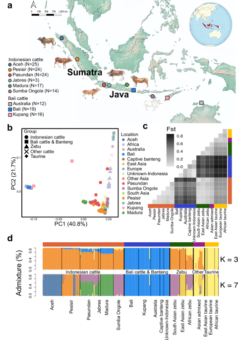
The research presented in this study complies with all relevant ethical regulations and was conducted in accordance with the Code of Conduct for Responsible Research of the University of Copenhagen. We collected 233 samples from 6 Indonesian cattle breeds (Aceh, Pesisir, Pasundan, Jabres, Madura, and Sumba Ongole), 3 Bali cattle populations (Bali, Kupang, Australia), and three individuals of Javan banteng from captivity in Texas, USA (Fig. 1a; Supplementary Data 1; Supplementary Data 2; Supplementary Fig. 1). The Bali cattle from Australia come from a feral population in Garig Gunak Barlu National Park in northern Australia, descended from 20 individuals that were released from an abandoned British outpost in 184932,56. Samples consisting of blood were kept in an EDTA buffer in the field, stored at −196 °C in dry shipper as soon as possible for transferring from the field to the laboratory in Bogor, and were further transferred to a −80 °C freezer for long-term storage. We then followed the manufacturer’s protocol instructions of the QIAGEN Blood and cell culture Kit to extract DNA. Before we did the default protocol, we added three treatment steps: (1) adding 500 µl of ice cold water to the blood samples, (2) centrifuge the diluted blood samples for 20 min with the speed of 17,900 x g in 4 °C, (3) discard the supernatant without disturbing the pellet. These extra steps were required to do the default kit protocol because of the humid climate in the Indonesian lab. Before using gel electrophoresis to check the quality of the genomic DNA, we further measured the DNA concentrations with a Qubit 2.0 Fluorometer and a Nanodrop. After DNA extraction, 1 mg genomic DNA was fragmented by Covaris (350 base pairs on average), followed by purification by AxyPrep Mag PCR clean-up kit. The fragments were end-repaired by End Repair Mix and then purified. The repaired DNA was combined with A-Tailing Mix, then the Illumina adaptors were ligated to the DNA adenylate 3’ ends, followed by product purification. Size selection was performed targeting insert sizes of 350 base pairs (bp). Several rounds of PCR amplification with PCR Primer Cocktail and PCR Master Mix were performed to enrich the adaptor-ligated DNA fragments. After purification, the size and quality of libraries was assessed by the Agilent Technologies 2100 Bioanalyzer and ABI StepOnePlus Realtime PCR System.

Additionally, we downloaded 81 publicly available, whole-genome sequencing datasets: 8 samples from Bali cattle from an unknown locality in Indonesia, 42 individuals of Bos indicus spreading from East Asia, South Asia, Latin America, and Africa, 27 individuals of Bos taurus from Asia, Middle East, Europe, and Africa, and two gaur (Bos gaurus), two Javan banteng (Bos javanicus) from zoological gardens (Supplementary Data 2; Supplementary Fig. 1).

Sequencing and mapping

All samples were sequenced using illumina paired-end 2 × 150 bp reads. This includes 230 samples sequenced to depth of 9.62X–17.0X coverage on Illumina NovaSeq platform and 3 samples from captive Javan banteng sequenced to depth of 15.9X–34.9X on the Illumina HiSeq2500 platform (Illumina Inc., San Diego, CA, USA). We assessed the quality of the raw reads using FastQC (bioinformatics.babraham.ac.uk/projects/fastqc) and MultiQC74 before mapping.

For mapping, we used a modified version of PALEOMIX BAM pipeline75 (github.com/xiqtcacf/IndonesianCattle-Scripts), which is a pipeline designed for the processing of demultiplexed, high-throughput, short-read sequencing data. We first trimmed Illumina universal adapters using AdapterRemoval v2.3.276. We merged read pairs with overlapping sequences of at least 11 bp to improve the fidelity of the overlapping region by selecting the highest-quality base when mismatches are observed. Mismatching positions in the alignment, where both read bases had the same quality, were set to ‘N’ via the ‘–collapse-conservatively’ option. We did not trim Ns or low-quality bases and only empty reads resulting from primer-dimers were discarded. We then mapped all trimmed reads using BWA-mem v0.7.17-r11887077 to two chromosome-level reference genomes: (1) BosTau9 (GenBank: GCA_002263795.2, ARS-UCD1.2), a female taurine from Hereford breed, and (2) Waterbuffalo (GenBank: GCA_003121395.1, UOA_WB_1), a female water buffalo from the Mediterranean breed. PCR duplicates were flagged using samtools v1.11 ‘markdup’ for paired reads and PALEOMIX ‘rmdup_collapsed’ for merged reads.

We merged the resulting BAM alignments from collapsed and paired reads for each individual, and filtered them based on standard BAM flags to exclude unmapped reads, reads with unmapped mate reads, secondary alignments, reads that failed QC, PCR duplicates, and supplementary alignments. We further excluded reads in alignments with inferred insert sizes <50 bp or >1000 bp, reads where <50 bp or <50% of the reads were aligned, and read pairs in which mates mapped to different contigs or not in the expected orientation. We finally generated statistics of the filtered BAM files by samtools ‘stats’ and ‘idxstats’78.

Sample filteringHeterozygosity

We excluded samples with extraordinarily high heterozygosity, because these samples likely suffer from DNA contamination or considerable sequencing errors. We calculated heterozygosity per individual based on site frequency spectrum (SFS) using genotype likelihood with the GATK model in ANGSD. The analysis revealed six individuals with excessively high heterozygosity (≥ 0.00620; Supplementary Data 2) and excluded five out of six for downstream analyses. We kept the sample with highest heterozygosity from Kupang (N_31B) as preliminary analyses suggested it might be a potential F1 hybrid.

Relatedness filtering

We removed duplicates and closely related samples using the methodology described in Waples et al. 79 We first computed the two-dimensional site-frequency spectrum (2d-SFS) for each pair of samples and then calculated three statistics from the 2d-SFS: R0, R1, and the KING-robust kinship coefficient. We found 54 duplicated pairs with KING-robust kinship > 0.460, of which most were from the Jabres breed, and 27 pairs of up to approximately second-degree relatives (KING-robust > 0.150). We excluded all but one sample with lower coverage from identified duplicated and related pairs, leading to 81 samples discarded (Supplementary Data 2).

Site filteringReference genome filtering

We implemented reference genome filtering based on different criteria. We used GenMap v1.2.080 to calculate the mappability score of each site of both the BosTau9 and the Waterbuffalo reference genomes, conservatively using 100 bp k-mers with up to two mismatches allowed (-K 100 -E 2), and default remaining settings. We removed all sites with a mappability score <1 for downstream analyses. We used RepeatMasker v.4.1.1 (repeatmasker.org) to identify repeat regions in both reference genomes, using ‘rmblast’ as the search engine and ‘mammal’ as the query species with default settings. We also excluded repeat regions identified by RepeatMasker, annotated sex chromosomes and scaffolds that were not assembled into chromosomes (Supplementary Data 3). Additionally, we inferred the sample sex using SATC81, based on the normalized sequencing depth on sex-linked scaffolds for each sample (Supplementary Data 2).

Global depth filtering

For each of the two mapping datasets, we estimated the global depth (read count) per site across all samples using the ANGSD command ‘-minMapQ 25 -minQ 30 -doCounts 1 -doDepth 1 -dumpCounts 1 -maxdepth 4000’ and then estimated the per-site median depth. We excluded sites with a global depth <0.5 times the median (0.5 × 1717 = 858.5) and >1.5 times the median (1.5 × 1717 = 2575.5) from all analyses (Supplementary Data 3).

Excess heterozygosity filtering

We removed regions with excessive heterozygosity, which is likely caused by problematic mapping due to repetitive or paralogous regions. We first generated a preliminary file of genotype likelihoods using ANGSD with the GATK model (-GL 2) from common polymorphic sites (MAF ≥ 0.05 and SNP p < 0.000001), base quality at least 25 (-minQ 25), and minimum mapping quality of 30 (-minMapQ 30). Using these genotype likelihoods as input to PCAngsd v0.98582,83, we then calculated the per-site inbreeding coefficients (F), ranging from −1 where all samples are heterozygous to 1 where all samples are homozygous, and performed a Hardy-Weinberg equilibrium likelihood ratio test accounting for population structure. The optimal number of principal components to model the population structure was inferred based on Velicer’s minimum average partial test84 implemented in PCAngsd. Finally, we removed windows of 10 Kb around sites with significant excessive heterozygosity estimates (F < −0.95 and p < 0.000001) based on the per-site inbreeding coefficients for both BosTau9 and Waterbuffalo reference (Supplementary Data 3).

Genotype calling and imputation

We performed genotype calling for both datasets mapped to BosTau9 and Waterbuffalo reference genomes using bcftools v1.1485. Genotype calling was only performed on the samples maintained after sample filtering and only on genomic regions retained after site filtering. We used the ‘bcftools pileup’ function based on reads with a minimum base quality of 25 and a minimum mapping quality of 30, enabling ‘-per-sample-mF’ to increase calling sensitivity. We then did genotype calling by using ‘–multiallelic-caller’. Finally, we removed both multiallelic sites and indels, and applied additional filtering using the setGT plugin of bcftools, imposing a minimum depth of coverage per site of 10 and only accepting heterozygous calls with at least 3 reads supporting each allele.

We did genotype imputation and phasing to remedy genotype missingness and refine the genotypes, because some samples had low depth for regular genotype calling. To prepare the input, we extracted bi-allelic SNPs from the genotype data mapped to both references: BosTau9, or ‘internal’ reference and Waterbuffalo, or ‘external’ reference. We did imputation and phasing using BEAGLE v3.3.286 separately for each chromosome. We visualized the distribution of genotype discordance between the original vcf and imputed vcf genotype files (Supplementary Fig. 30a). In order to evaluate the accuracy of imputation, we additionally conducted the analysis by downsampling the highest-depth banteng individual (34.86X, LIB112407_Banteng_85B_Texas) to depths 1X, 5X, 10X, then imputing them, and comparing the imputed genotypes with the high-quality genotype calls for the full data from this sample using an R package ‘vcfppR’87. The analysis showed a very high concordance between imputed genotype calls and true genotype calls, supporting the accuracy of imputation (Supplementary Fig. 30b).

PCA and admixture analyses

To investigate population structure, we used HaploNet29, which implements a neural network on local clustering of phased data. We trained the HaploNet model using default settings and produced log-likelihoods that can be processed further to PCA and Admixture. We used ten eigenvectors to capture population structure between and within the filtered dataset of 231 individuals (without the two gaurs) mapped to BosTau9. For the admixture analysis, we set the number of ancestry (K) from 3 to 12, with 50 independent runs for each K. We used a convergence criterion of reaching within 5 log-likelihood units of the lowest log-likelihood in at least 3 independent replicates. We obtained convergence with K from 3 to 7. Based on the HaploNet results at K = 7 we then defined a subset of individuals as non-admixed representatives of each breed or population by removing samples that contained > 10% of admixture from a different ancestry source than the population majority.

Genetic diversity, runs of homozygosity, and population differentiationHeterozygosity

We assessed genetic diversity of cattle based on genome-wide individual heterozygosity, using filtered genotype-called data that included non-variable sites with a range of depth from 6 to two times of average depth of each sample, a minimum allelic support of 3, a minimum mapping quality of 30, and a base quality of 25. We calculated the individual heterozygosity as the number of heterozygous genotypes relative to the number of total sites.

Runs of homozygosity

We first explored various different approaches and data filtering options to optimize the detection of runs of homozygosity (ROHs) in each individual. For assessment and validation, we visualized ROHs across the genome similar to the approach in Liu et al. 38 and checked visually the performance of ROH calling under different filtering and PLINK detection settings. The assessment criteria include looking for signs of long apparent ROHs being broken up, and the ability of smaller regions of consistently reduced heterozygosity to be called as ROHs in the analysis. Based on these analyses, we used the imputed datasets mapped to BosTau9 to estimate ROHs using PLINK v1.90b6.24. In PLINK we applied maximum heterozygous calls of 5 (–homozyg-window-het 5), a minimum of 500 kilobases for a ROH (–homozyg-kb 500), and filtered out all variants with missing calls (–geno 0). We merged distinct ROHs within 100 Kb distance, and categorized all resulting ROHs into five length groups: 0.5–1 Mb, 1–2 Mb, 2–5 Mb, 5–10 Mb, and >10 Mb.

Global F
ST

To infer population differentiation, we calculated genome-wide global FST for each pair of populations (after removing admixed individuals) using ‘–fst’ implemented in PLINK2.088. This calculates Hudson’s FST estimator, which is robust to differences in sample size between populations89. We further built a NeighborNet tree based on the pairwise global FST distances in order to show the relationships of the populations.

Population history and introgression analysisTreemix

To investigate the history of population splits and historical admixture events, we performed a TreeMix analysis90 using the imputed data mapped to the Waterbuffalo reference. Because relatedness can underestimate covariance and lead to spurious inferences of migration using Treemix, we did a more stringent sample filtering for the input datasets by applying a threshold of KING kinship coefficient of 0.1 to exclude potentially second degree of related samples. In the TreeMix analysis we included the Indonesian cattle breeds, Bali cattle, captive banteng, East Asian zebu, East Asian taurine and European taurine, two gaurs, and the Waterbuffalo to root the tree (Supplementary Data 2). We ran TreeMix assuming 0–10 migration events. For each number of migration events (m), we ran 100 iterations using bootstrap (-bootstrap) and a block size of 1000 SNPs (-k 1000). We inferred the final, optimal number of migration edges (m) from the second-order rate of change in likelihood (Δm) weighted by the standard deviation using the ‘Evanno’ method implemented in OptM91.

D-statistics

To infer the evolutionary relationships and ancient admixture events, we calculated D-statistics (Patterson’s D, also called ABBA-BABA) using the R package ADMIXTOOLS292. We used datasets mapped to the Waterbuffalo reference to mitigate the effects of reference bias. We ran D-statistics analyses of the type (H1-H2-H3-H4) with both topology of captive banteng-cattle-South Asian zebu-water buffalo and cattle-South Asian zebu-captive banteng-water buffalo, using the function ‘qpdstat’ implemented in ADMIXTOOLS2.

mtDNA, Y-chromosome DNA analyses, and phylogenetic tree

To infer maternal and paternal phylogenetic relationship between cattle, we inferred the phylogenetic tree for both mitochondrial DNA (mtDNA) and Y-chromosome (Ychr). To identify the matrilines in the cattle, we generated consensus mitochondrial sequences. Briefly, we used the -doFasta 1 option of ANGSD93 with quality values specified as ‘-minMapQ 30 -minQ 30 -setMinDepth 5 -uniqueOnly 1 -remove_bads 1’ and also ‘-doCounts 1’ to generate consensus fasta from whole-genome sequencing data mapped to BosTau9 mitochondrial scaffold (NC_006853). We aligned these fasta sequences using the FFT-NS-1 (fast) option of MAFFT94. We imported the aligned sequences into Jalview alignment editor95 and removed the regions in the alignment with high ‘N’, and exported the edited sequence in fasta format. We then aligned these edited sequences using the G-INS-i (accurate) option of MAFFT and wrote the output in fasta format. For creating a haplotype network, we converted the fasta files to nexus format and imported to POPART96 to create a minimum spanning haplotype network with an epsilon 0. For creating a neighbor-joining tree, we imported the aligned sequences to TreeViewer97 and used a Hamming distance model with 5000 bootstrap replicates.

We built the phylogenetic tree for the Y chromosome (Ychr) using BEAST v1.10.498. We first generated the consensus Ychr (only in males) sequences using ANGSD from whole-genome sequencing data mapped to taurine Ychr (GenBank: CM001061.2), with the same settings as for mtDNA consensus sequences. We removed heteroplasmic sites by masking (as ‘N’) any Y chromosome site where <95% of reads carried the same base. After consensus calling, we then performed phylogenetic analyses using the GTR + G + I substitution model and a coalescent Extended Bayesian Skyline Plot prior to avoid restricting the tree by imposing a confining demographic prior. We then ran the Markov chain-Monte Carlo (MCMC) chain for 107 steps, sampling trees and parameters every 1000 steps. We assessed convergence and proper mixing by visual inspection and by estimating parameter effective sample sizes using TRACER99. We used TreeAnnotator100 to make a maximum clade credibility tree, discarding the first 1000 trees. We used Figtree v1.4.4 (tree.bio.ed.ac.uk/software/figtree) to visualize the maximum clade credibility tree.

Divergence time

We used MSMC2101 to estimate the divergence time between zebu (Bos indicus), banteng (B. javanicus) and Bali cattle. We used the phased callable regions of two individuals per population, randomly sampling 10 million SNPs from the genome. We scaled the results for visualization by assuming a generation time of 5–7 years4,43,44, and a mutation rate of 1.26 × 10−8 generation4.

Local ancestry inference in admixed populationsLOTER

After having identified cattle populations with signs of ancestral admixture, we did local ancestry inference using LOTER39. LOTER has been used for a wide range of species such as humans102,103, primates104,105, cattle7, and rapeseed106, and does not require prior knowledge such as recombination maps to be implemented. We used imputed and phased datasets with a total of 22,158,517 SNPs mapped to BosTau9 as input for LOTER. We used unadmixed zebu and banteng individuals as two ancestry source references: (1) the zebu reference population consisted of 14 Sumba Ongole and 11 South Asian zebu, and (2) the banteng reference population consisted of 19 Bali cattle from Bali, 12 Bali cattle from Australia, and five captive banteng. In the reference sets we considered that a low probability of being admixed was more important than having a larger reference set of individuals with more uncertain admixture profiles. We used a total of 90 individuals as target admixed individuals from the following populations with introgression from banteng or another Bos source: Aceh, Pesisir, Pasundan, Jabres, Madura, and East Asian zebu. In addition, we included Bali cattle from Kupang, because this population showed signs of introgression from cattle. We performed all analyses using the ‘lc.loter_smooth’ function, which enables a phase-correction module. We estimated the overall proportion of banteng ancestry in each individual by calculating the number of SNPs inferred to be derived from banteng and dividing by the total number of SNP sites. Afterwards, we used non-overlapping sliding windows of 50 Kb to consolidate the raw output from LOTER across individuals in each population. For each admixed population, we calculated the proportion of banteng ancestry in each 50 Kb window by calculating the proportion of SNPs inferred to be of banteng ancestry in each individual (two haplotypes per individual), and taking the mean of this value across all haplotypes in the population.

As local ancestry inference can potentially be affected by the choice of reference genome we assessed whether mapping to a banteng reference would impact the LOTER analyses. We downloaded a recently available banteng reference genome (RefSeq: GCF_032452875.1, ARS-OSU_banteng_1.0) and performed mapping of all the raw data as described above to this reference genome. We then redid all steps described above in the “Site filtering” and “Genotype calling and imputation” sections separately for this alternative mapping, and performed a LOTER analysis as described above. Finally, we calculated the genome-wide proportion of inferred banteng ancestry based on this alternative mapping and plotted the count of SNPs inferred to be of banteng ancestry in each 50 Kb genomic window for each of the two mapped data sets, for two example individuals from Madura (N_911 and N_935). Comparability between the two mapped data sets was ensured by exploiting a liftover of genomic coordinates between the banteng and cattle reference genome, available on NCBI. The analyses found almost identical genome-wide banteng proportions using either mapped data set (Madura population as example shown in Supplementary Fig. 18a), and that the correlation between banteng-inferred SNPs across individual windows was also very high (Supplementary Fig. 18b). We therefore conclude that our findings are robust to the choice of reference genome.

F4 ratios

To estimate the ancestry proportions in each admixed individual, we calculated F4 admixture ratios using ‘qpadm’ implemented in ADMIXTOOLS292. This models a target population as a mixture of two source populations given a set of outgroup populations40. We used the same ancestry source references and target admixed populations as in the LOTER analysis. We then estimated F4 ratios in the form of α = f4 (taurine, water buffalo; banteng source, target) / f4 (taurine, water buffalo; banteng source, zebu source). We used 5 × 106 as the SNP block size for jackknifing.

Hmmix

Additionally, we detected the segments of individual genomes of archaic introgression on Indonesian cattle (Aceh, Pesisir, Pasundan, Jabres, Madura) and East Asian zebu population, with South Asian zebu and Sumba Ongole as outgroups using Hmmix v0.6.941. This approach is based on a hidden Markov model that identifies genomic regions with a high density of single nucleotide variants not seen in outgroup populations (non-admixed); therefore, it can be used without relying on ancestry reference sources. The rationale behind this approach is to identify regions of high SNP density after removing variation found in outgroup populations, because introgressed regions with higher SNP density have spent more time accumulating variation that is not found in the outgroup compared to non-introgressed regions. We first prepared the input files for this method from imputed datasets mapped to BosTau9 using the sites retained after site filtering as weights, local mutation rates, and individual observation files using scripts provided with the repository for Hmmix (github.com/LauritsSkov/Introgression-detection). We then applied the method to Indonesian cattle and East Asian zebu populations using the following different prior parameters as model training to detect the best-fitting hidden Markov model parameters: Aceh (starting_probabilities = 0.93, 0.07, transitions = 0.98, 0.02 and 0.25, 0.75, emissions = 2, 25); Pesisir (starting_probabilities = 0.88, 0.12, transitions = 0.99, 0.01 and 0.09, 0.91, emissions = 2, 25); Pasundan (starting_probabilities = 0.80, 0.20, transitions = 0.99, 0.01 and 0.05, 0.95, emissions = 2, 25); Jabres (starting_probabilities = 0.76, 0.24, transitions = 0.99, 0.01 and 0.04, 0.96, emissions = 2, 25); Madura (starting_probabilities = 0.63, 0.37, transitions = 0.98, 0.02 and 0.04, 0.94, emissions = 2, 25); East Asian zebu (starting_probabilities = 0.84, 0.16, transitions = 0.93, 0.07 and 0.36, 0.64, emissions = 2, 25). Subsequently, we decoded the data with the best hidden Markov model parameters that maximized the likelihood and identified the archaic introgressed segments. We annotated the archaic introgressed regions by potential source populations (or species) by calculating the ratio of inferred archaic SNPs in each archaic fragment that was shared with each of two possible source populations: 1) a banteng population consisting of five Javan banteng, 19 Bali cattle from Bali, and 12 Bali cattle from Australia, and 2) two gaur individuals. Moreover, we calculated the identity-by-state matrix for all pairs of admixed cattle individuals based on their overlapping archaic regions. We did all analyses using a 10 Kb window and retaining only the archaic regions with probability >0.9.

U
X and related analyses

We also explored a metric proposed by Racimo et al. 107 to identify putatively adaptively introgressed regions. The metric tabulates the sites that are nearly fixed for different alleles in cattle and banteng (banteng-specific alleles), and where the banteng-specific allele occurs at a high frequency in the admixed population. Known as the UA,B,C(w,x,y)107 statistic, where w = the maximum allele frequency in unadmixed cattle, x = minimum allele frequency in the target admixed population, and y = the minimum allele frequency in banteng. We calculated both UA,B,C(0.05,0.50,0.95) and UA,B,C(0.05,0.20,0.95) in non-overlapping, 50 Kb windows in each admixed population. We used the same reference populations to represent unadmixed zebu and banteng as in the LOTER analysis. For practicality, we refer to these statistics as Uabc50 and Uabc20, respectively. However, it is challenging to decide on the value of minimum allele frequency x in population B that gives the best discriminative power for adaptive introgression107, and we found that this problem is exacerbated when the original admixture proportions as well as sample sizes differ among populations. In addition, this count statistic is influenced by the genome-wide variation in absolute sequence divergence between populations A and C, leading to a potential decoupling of the UA,B,C count from the proportion of local ancestry. Therefore, we also calculated another statistic (UX) by calculating x in UA,B,C(0.05,x,0.95) for each admixed population in 50 Kb bins. In other words, we calculated the mean allele frequency of population B in sites that had <0.05 derived allele frequency in unadmixed cattle, and >0.95 across Bali cattle and banteng. This mean allele frequency in banteng-diagnostic sites UX has a more continuous distribution than Uabc20 and Uabc50, and had a higher correlation with local LOTER and Hmmix ancestry proportions than any of the UA,B,C we examined, but still constitutes an independent approach for inferring regions of high banteng ancestry in admixed cattle.

Correlation between banteng ancestry and genomic features: recombination rates, coding region density, and conservation score

To investigate correlations between genomic features and banteng ancestry in admixed breeds, we compared the estimated proportion of banteng ancestry in each 50 Kb window with the mean recombination rate, the mean coding region density, and the number of conserved sites in the same window for the Madura population. For recombination rates, we obtained a sex-specific cattle recombination map108 and did linear interpolation for each SNP by using the ‘approx’ function in R. We then aggregated the recombination map to the 50 Kb window for both sexes. We also obtained information regarding the number of sites in coding regions and the number of conserved sites (phastCons30way) from the Ruminant Genome Database (RGDv2109) binned to the same window size. The latter was based on the BosTau9 version of the Bos taurus reference genome collated with the Y chromosome of the Btau5.0.1 version (ARS-UCD1.2_Btau5.0.1). For each comparison, we split the windows into 10 quantiles and then calculated the mean proportion of banteng ancestry for each quantile along with its standard error as a measure of uncertainty. We plotted the distributions across quantiles as both scatter plots overlaid with the means, as well as kernel density plots. We also applied a genome-wide Spearman rank correlation test of banteng ancestry proportions among each pair of admixed breeds across all windows and those in the top 5%.

Ancestry-specific population structure in admixed populations

To investigate each of the ancestry sources in admixed populations, we inferred population structure for zebu-specific and banteng-specific ancestry regions, using EMU, a method designed to be robust to both random and non-random missingness110. We used imputed datasets mapped to BosTau9 and performed a stringent-sample filtering by removing one of each pair of K1 > 0.2 identified by NgsRelate111,112 within each population (Supplementary Fig. 31). For inferring zebu ancestry structure, we first extracted SNPs inferred to be of zebu ancestry by LOTER per individual, and regions identified as ‘cattle’ by Hmmix per individual. We then merged all admixed individuals with LOTER-zebu and with Hmmix-zebu ancestry with the unadmixed zebu population (Sumba Ongole and South Asian Zebu) separately as inputs for EMU analyses. To infer population structure with EMU, we applied seven eigenvectors (–n_eig 7), maximum iterations of 1000 (–iter 1000), and a threshold for minor allele frequencies of 0.05 (-f 0.05). We estimated PCA for banteng ancestry structure in a similar way to inferring zebu ancestry by extracting SNP positions with banteng ancestry using LOTER and regions with ratio > 0.8 (number of banteng population SNPs ÷ derived number of SNPs) of Hmmix per admixed sample, respectively. EMU-PCA was then performed on this set of banteng annotated ancestry regions in admixed individuals and the whole genome of unadmixed banteng populations (Bali cattle from Bali, Bali cattle from Australia, and captive banteng) using the same settings as above, except for eight eigenvectors (–n_eig 8).

As some additional whole-genome sequenced samples from Asian zebu became available during the preparation of the study that could potentially be of relevance to place the masked zebu ancestry of the Indonesian cattle into a geographical context, we downloaded data from Chen et al.113 and Chen et al.5 (Supplementary Data 7) and performed mapping, imputation and LOTER analysis as described for our original data set. We then included them in an additional EMU-PCA. These samples were placed on a cline towards the East Asian zebu samples in the zebu-specific EMU-PCA, consistent with their geographical placement in northernmost Southeast Asia along the shortest route between India and China (Supplementary Fig. 11b). While supporting the credibility of the EMU-PCA as a method to detect historical dispersals, this result does not enable us to further disentangle the origin of zebu cattle introduced to Indonesia. Only samples from further south in mainland Southeast Asia would have enabled this.

To check the performance of masking based on LOTER results, we performed a check by recalculating D-statistics after masking all SNPs inferred to be introgressed in each sample. This plot demonstrates the ability of the LOTER based masking to remove all or by far most of the introgression from banteng-like Bos sources (Supplementary Fig. 11a).

Estimation of admixture time

To infer the timing of admixture events, we traced the ancestry of discrete genomic segments for all of Indonesian cattle populations and East Asian zebu using Ancestry_HMM, a hidden Markov model-based method42,45. We fitted a single-pulse admixture model to the genome-wide variation data and used the mean ancestry proportions estimated by LOTER as the assumed admixture proportion (-p 1 100000 -0.6 -p 0 -500 -0.4). We also tried a two-pulse admixture model for the Javan breeds with the settings: ‘-p 1 100000 -0.6 -p 0 -1000 -0.2 -p 0 -200 -0.2’. However, the higher admixture time and lower admixture (~ 0.01%) estimated for the first pulse when using the two-pulse model suggests that the two-pulse model is a poor fit to the data45 (Supplementary Fig. 32). We quantified uncertainties by doing 100 bootstrap replicates for each population using a block size of 5000 SNPs (-b 100 5000).

Overlapping introgressed segments among LOTER, Hmmix, and U
X

To obtain the top 5% windows of highest-inferred banteng ancestry in each of the five cattle groups (Aceh, Pesisir, Pasundan, Madura, and East Asian Zebu), we merged the results from LOTER, Hmmix, and UX using non-overlapping 50 Kb windows made according to the taurine autosomal chromosomes (BosTau9) and annotated with genes coming from BosTau9 reference-genome annotation (GFF, Ensembl version 106) using bedtools intersect114. For each of the 50 Kb windows, we counted the proportion of banteng SNPs coming from LOTER (anc1), number of SNPs in UX, and the mean proportion of archaic regions with probability ≥ 0.9 from Hmmix. For each statistic, we determined the top 5% quantile from each cattle group to filter out windows that do not contain the highest banteng ancestry. Due to the high number of windows with Uabc50 and Uabc20 = 0, the top 5% quantile from UX statistics are 0 and hence not used for this filtering step. Before obtaining the top 5% windows of highest banteng ancestry, we first fitted a linear model to explore the predictive power of Hmmix for LOTER and found that Hmmix can explain more than 50% of the variation in LOTER values (Supplementary Fig. 23). However, consistently higher proportion of introgressed ancestry inferred by Hmmix than by LOTER and Ux, could potentially be due to either Hmmix finding introgression from a wider array of sources than LOTER (e.g. other bovines present in SEA), or to a higher tendency of false positives in Hmmix, or a mixture of the two. We thus only kept windows that passed the top 5% quantile of LOTER values in each cattle group. We then listed these regions for each cattle group and annotated them with a gene list of BosTau9 from NCBI Bos taurus Annotation Release 106 (2019-12-18, GCF_002263795.1_ARS-UCD1.2_genomic.gff.gz115) and QTL information of Bos taurus ARS-UCD1.2 from QTLdb release 53116 to identify signs of adaptive introgression. We used values from Hmmix and UX for further validation as an overall sanity check, or robustness analysis.

Gene enrichment analysis

To characterize the functional associations of these candidate regions for adaptive introgression, we performed GO-enrichment analyses for the outlier gene set from each breed. For each unique gene in the top 5% list, as well as genes in the zero-banteng regions, we performed an overrepresentation analysis for gene-enrichment by using the g:GOSt feature of the web-based g:Profiler117. Genes overlapping the top 5% banteng ancestry regions of each cattle population (Aceh, Pesisir, Pasundan, Madura, and East Asian zebu) were used as input to g:GOSt v110 using Bos taurus as the annotation set and a g:SCS significance threshold of 0.05. For each cattle population we collected the outcome of the gene enrichment based on molecular function, cellular component, biological process, as well as terms from KEGG, REAC, and HP if any (Supplementary Data 8). We then made an UpSet plot for genes in the top 5% using the ComplexUpset package118 in R v4.3.3119 to see how many outlier genes were shared across multiple cattle populations. To assess any overall overrepresentation or underrepresentation of genes contained in the top 5% banteng ancestry regions in each breed, we performed a simulation by randomly choosing 1000 times 5% of the genomic windows (2482 windows) out of the total of 49,624 genome-wide windows. We then counted the number of genes for each iteration and plotted the results in a histogram.

Haplotype structure

We visualized haplotype structure of the ASIP gene on chromosome 13 between 63.64 Mb and 63.67 Mb using Haplostrips120. The software extracts the haplotype data from the phased genotypes, keeps the samples belonging to populations of interest and chooses only the most informative sites by eliminating variations with very low frequency in all the populations, and finally produces a plot that displays the haplotypes in rows while each column represents a SNP within a region of interest. Populations of captive banteng and Bali cattle were lumped as banteng and were treated as the reference population. We also built the haplotype network for ASIP gene using the same methods described above for inferring mtDNA phylogenetic tree.

Reporting summary

Further information on research design is available in the Nature Portfolio Reporting Summary linked to this article.