
Birefringent characteristics of mica substrates
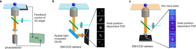
The critical factor for the performance of the feedback-free (i.e., scan-free) single-particle 3D tracking is PSF engineering because the 3D coordinates of the particle are determined by the axial-position dependent fluorescence pattern. Various PSF engineering methods covering different focal ranges have been reported31. Inserting an SLM in the detection optical path is the most common way to engineer the PSF. In theory, PSF engineering can also be done using optical materials with anisotropic optical characteristics as a substrate to mount microscope specimens.
Mica is an optically semi-transparent, birefringent material with potential applications in PSF engineering. While mica is commonly used as a substrate for atomic force microscopy measurements because it can provide an atomically flat surface, its application in optical microscopy has been limited32. This limitation arises from the complex optical properties of biaxial birefringence33,34, which significantly alter fluorescence images captured through the substrate. To date, the effects of mica’s biaxial birefringence on image formation in optical microscopy have not been systematically explored. Consequently, mica substrates have not been utilized for PSF engineering. Biaxial birefringence is known for its unique optical effect of conical refraction, and in recent years, it has regained attention for applications in optical trapping, free-space optical communications, polarization metrology, super-resolution imaging, two-photon polymerization, and various laser applications35.
Both excitation light (Fig. 2) and emitted fluorescence (Fig. 3) propagating through the mica plate are affected by its birefringence, characterized by an anisotropic refractive index. The mica usually comes in the form of a thin plate, with the surface being the (001) plane with crystal cleavage properties (Fig. 2a). It has a negative acute bisectrix of optical biaxial nearly matching the norm of cleavage surface with the shift of 3 to 5°33,36. Therefore, the direction of the optical biradial of a thin mica substrate placed on a microscope aligns nearly coaxially with the optical axis of the microscope. Optical biaxial crystals can be described as three components of distinct refractive indices along the optic principal axis. The collimated light propagating through a thin mica substrate perpendicularly to the cleavage surface of (001) can be approximated using two effective reflective indices of nβ and nγ (Fig. 2a). The differences between these refractive indices cause phase retardation between the light components vibrating along these principal optic axes. The intensities of two polarization components of the light transmitted through a thin mica plate are thus modulated with the rotation angle (θ) of the mica plate about the Z-axis (Fig. 2b, c). The effective birefringence of the mica plates in our experimental configuration \(\left({\delta }_{\gamma -\beta }={n}_{\gamma }-{n}_{\beta }\right)\) was determined by the mica substrate thickness-dependent retardation effect on the transmitting light (Fig. 2c, see Methods and Supplementary Methods for details). The effective birefringence of mica used in this study was determined to be δγ-β = 5.24 × 10⁻³ at 532 nm, the average of result from multiple mica plates with different thicknesses. The mica thickness-dependent retardation obtained from the δγ-β value is shown in Fig. 2d.
Fig. 2: Effect of the birefringence of the mica substrates on excitation light.
a Schematic illustration of the birefringent characteristics of mica. α, β, and γ represent the principal optic axes of mica with refractive indices of nα, nβ, and nγ, respectively. a, b, and c are crystallographic axes. b Schematic illustration of the optical path of an excitation laser in a wide-field fluorescence microscope. The mica substrate has a thickness of d. β and γ represent the principal optic axes of the mica substrate. θ is the rotational angle of the mica substrate. c Transmittance of the 532 nm light through the mica substrate with different thicknesses. The solid line shows the fitting of the data to Eq. 3. d Thickness-dependent retardance of the mica substrates. e Schematic illustration of the polarization states of the excitation light that passes through the mica substrates. A linearly polarized excitation light passes through the mica substrate with its polarization direction parallel (left) and non-parallel (right) to one of the optic axes of the mica substrate.
Fig. 3: Effect of the birefringence of the mica substrates on the image formation in wide-field fluorescence microscopy.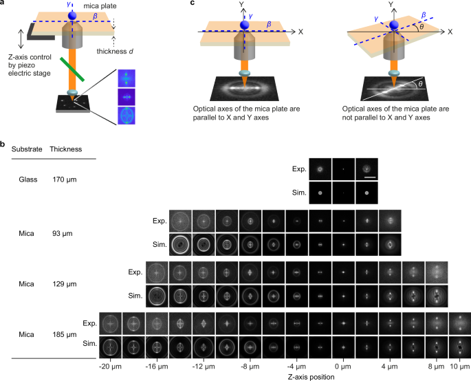
a Schematic illustration of the image formation of the fluorescence emitted by a fluorophore located close to the mica substrate. The mica substrate has a thickness of d. β and γ represent the principal optic axes of the mica substrate. b Experimentally obtained (top) and simulated (bottom) fluorescence images of the 60 nm fluorescent nanospheres captured at varied Z-axis positions through a glass substrate and the mica substrates with 110 µm, 170 µm, and 185 µm thickness. The Z-axis position of 0 µm was defined by the fluorescence image with the smallest spot size. PSF patterns obtained from three independent experiments were compared in each mica substrate thickness to ensure reproducibility. Scale bar = 10 µm. c Effect of the orientation of the mica substrate on the image formation. Fluorescence images of the 60 nm fluorescent nanospheres were captured through the mica substrate with its optic axes β and γ parallel (left) and non-parallel (right) to the X and Y axes of the imaging experiment. θ represents the angle between the optic axes of mica β and the X axis.
Because of the thickness- and wavelength-dependent retardation effect, a polarization state of the excitation light passing through mica substrates could be modified depending on its thickness or rotation (Fig. 2b). In order to unify the excitation conditions that are independent of the thickness of the mica substrate and the excitation wavelength, we used a linearly polarized light whose polarization direction aligned with one of the principal optic axes of mica (Fig. 2e). This excitation configuration guarantees the sample to be excited under the same linear polarization condition, regardless of the thickness of the mica substrates and the wavelength of the excitation laser.
PSF engineering using mica substrates
The birefringent characteristic of mica substrates also affects the image formation of the fluorescence emitted by a fluorophore located close to it (i.e., modification of the PSF, Fig. 3a). Fluorescence images of 60 nm fluorescent nanoparticles deposited on a 170 µm-thick glass coverslip captured at different axial positions through a high numerical aperture (NA) microscope objective lens clearly showed concentric patterns, whereas images of the same fluorescent nanoparticles captured through the mica substrates showed axial-position-dependent non-concentric patterns (Fig. 3b). We found that the mica substrates with different thicknesses exhibited axial-position-dependent pattern change over different axial axis ranges (Fig. 3b). Notably, the pattern change was observed over the 30 µm axial range (Fig. 3b and Supplementary Fig. 1). We note that the Z-axis position of 0 µm was defined by the fluorescence image with the smallest spot size (Supplementary Note 1). The mica substrate with 185 µm thickness gave the largest axial range with a relatively high signal-to-background ratio (Fig. 3b). We obtained similar axial-position-dependent pattern change for the 488, 532, and 640 nm excitation conditions (Supplementary Note 2). Since the magnification and NA of the objective lens also affect the PSF formed through the mica substrates (Supplementary Fig. 2), we conducted our imaging experiments with consistent conditions (i.e., an objective lens with 100× magnification and 1.49 NA).
The PSF along the XY plane obtained through the mica substrate is approximately half the size used in the 3D tracking method that covers the largest axial range reported previously over the entire axial range (Supplementary Figs. 3 and 4, Supplementary Table 1). In addition, the rotational orientation of the mica substrate (i.e., the orientation of optic axes) affects the orientation of the generated PSF (Fig. 3c). Thus, we adjusted the orientation of the two optic axes of the mica substrate to the X- and Y-axis of the imaging setup (Fig. 3c, Supplementary Note 3). We also confirmed that mica substrates with the same thicknesses (within 4% error37) give virtually identical PSF (i.e., the same Z-position-dependent fluorescence pattern) and that the PSF generated through mica substrates are stable over an extended period of time under varying conditions (e.g., temperature and moisture, Supplementary Note 4). However, we note that mica substrates obtained from different origins might provide slightly different PSFs as muscovite mica is known to have a variation in optical properties (e.g., refractive index, absorbing spectrum33, see below).
Simulation of the engineered PSF generated through mica substrates
To verify that the birefringent characteristic of the mica substrates causes the observed PSF modifications, we performed a simulation of the PSF and examined the effect of the biaxial birefringent substrates on the formation of the PSF. The PSF simulation was carried out by employing optical Fourier processing (see Methods and Supplementary Methods). The PSF calculated for the standard substrate (i.e., a glass substrate with 170 μm thickness) showed a diffraction-limited spot at the focal point, whereas concentric spatial patterns were observed at the Z-axis position 2 μm away from the focal point (Fig. 3b), consistent with the experimentally observed PSF. Next, we calculated PSF under the same conditions but replacing the standard substrate with a biaxial birefringent substrate with varied thickness. The optical axis of the microscope was aligned with the normal direction to the (001) plane (Fig. 2a), and the three refractive indices for each optic axis reported for muscovite mica were used for the simulation. The simulated PSF exhibited an axial position-dependent non-concentric pattern (Fig. 3b). Importantly, the simulated patterns agree excellently with the experimentally obtained patterns in the entire axial axis range. In addition, our simulation nicely reproduces the axial-position-dependent pattern change over different axial axis ranges observed for the mica substrates with different thicknesses (Fig. 3b). These results confirm that the modifications of the PSF originate from the biaxial-birefringent optical characteristic of mica.
Our simulation also indicated that the PSF modification by mica substrates might be sensitive to the value of three refractive indexes. We compared four different combinations of reported refractive indexes for muscovite mica from different origins38. The PSF generated through the mica substrate is similar to the simulated PSF generated through muscovite mica obtained from different sources (Supplementary Fig. 5), suggesting that there is no need to experimentally measure the refractive indices of a mica substrate prior to the imaging experiment. The PSF simulation also suggests that the axial-position-dependent patterns generated through the mica substrates are almost identical in a thickness range of 165–185 μm (Supplementary Fig. 6), and thus, we arbitrarily chose the mica substrates within this thickness range for the experiments we reported in this study. We also simulated the PSF formation through the different optic axes of the mica substrate. The axial position-dependent patterns similar to the experimentally observed ones were obtained only when the optical axis of the microscope was aligned with the normal direction to the (001) plane (i.e., optical biradial of the substrate) in the simulation (Supplementary Fig. 7, Supplementary Note 5).
Single-particle 3D localization using the PSF
Using the axial position-dependent PSF imaged through the mica substrates, we determined the 3D coordinate of a single emitter. We recorded reference PSF images of a fluorescence nanoparticle at pre-defined axial positions. The 3D coordinates of the target nanoparticles were determined by finding the best-matched reference PSF images. This was done by performing a normalized 2D cross-correlation analysis (see Methods for details).
We experimentally determined the precision of 3D localization by localizing 60 nm fluorescent nanoparticles deposited on a mica substrate coated by poly(dimethylsiloxane) thin film (Fig. 4a; see Methods for the details). The localization precision was estimated by the standard deviation of the localized 3D coordinates. While the precision of the axial-position determination is limited by the z-axis interval distance of the reference PSF images, the precision of XY coordinates determination is restricted by the pixel size of the recorded images. The 3D localization precisions (i.e., standard deviations of the localizations) determined at different axial positions with the reference images captured at the 50 nm step size and the image pixel size of 83 nm are shown in Supplementary Fig. 8. The localization precisions along the X, Y, and Z coordinates obtained under these imaging conditions are better than 50 nm in the Z-axis range of 18 µm (Supplementary Fig. 8). The large axial position-dependent variation in the 3D localization precision was observed, indicating that the localization precisions are significantly affected by the z-axis interval distance of the reference PSF images and the pixel size.
Fig. 4: 3D localization precision of the birefringence-based point spread function engineering.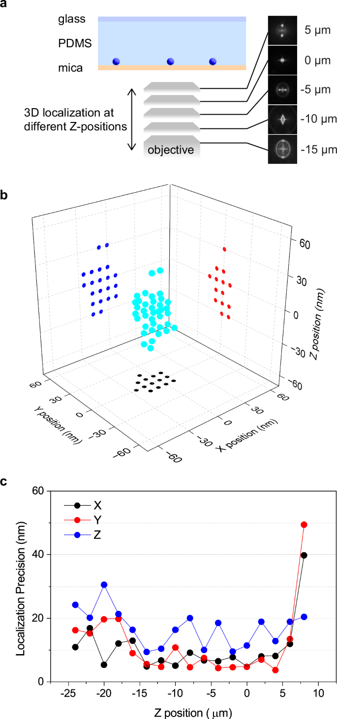
a A schematic illustration of the experimental configurations. 60 nm fluorescent nanospheres deposited on the mica substrate were embedded in a thin film of polydimethylsiloxane (PDMS). This experiment was conducted using a 185 µm-thick mica substrate. b A typical example of localized 3D coordinates (cyan) with projection to XY (black), XZ (blue), and YZ (red) planes. c Z-axis position-dependent 3D localization precision. The Z-axis position of 0 µm was defined by the fluorescence image with the smallest spot size.
We further conducted a similar 3D localization experiment with a smaller axial step size of the reference PSF images (10 nm interval) and sub-pixel localization in the XY directions (see Methods for the details). A typical 3D localization plot is displayed in Fig. 4b. The 3D localization precisions were greatly improved by reducing the axial interval distance and adapting sub-pixel localization, which gave the 3D localization precisions higher than 30 nm in the Z-axis range of 32 µm (Fig. 4c). Both the axial range (32 µm) and 3D localization precision (higher than 30 nm) achieved using our method surpass those reported in the literature (20 µm axial range with 50 nm theoretical localization precision)19.
Effect of the emitter-to-mica substrate distance on the axial position localization
We examined the effect of the distance between the emitters and the mica substrate on the formation of the PSF pattern and, therefore, the 3D localization accuracies for the emitters located at different axial positions from the mica surface. This was done by preparing a thin film sample with a wedge shape sandwiched between glass and mica substrates, on which fluorescent nanoparticles are deposited (Fig. 5). We first recorded fluorescence images of the nanoparticles deposited on both surfaces at different axial positions through the glass substrate (Fig. 5a, b). The axial positions of the two nanoparticles were determined by finding fluorescence images with minimum spot sizes from which the distance between the two nanoparticles on both surfaces was determined (Fig. 5b). Next, we flipped the sample and captured fluorescence images of the nanoparticles deposited on both surfaces at different axial positions through the mica substrate (Supplementary Fig. 9). The images were captured at different X-axis positions along the line region, which is the same as the one used in the imaging experiment through the glass substrate (Fig. 5c, d). The distances between the two surfaces were determined by finding the fluorescence patterns corresponding to the same axial positions (e.g., the images corresponding to 0 µm axial position, Fig. 5d). The distances between the two surfaces determined by the fluorescence patterns observed through the glass and mica substrates at different sample positions (i.e., different X-axis positions) are shown in Fig. 5e. The distance versus sample position plots (Fig. 5e) obtained from the images captured through the glass and mica substrates were fitted to a linear function with slopes of −1.36 (glass) and −1.43(mica). The nearly identical fitted lines for the two plots demonstrate that the gap distances between the two substrates, and, therefore, the axial positions of the fluorescent nanoparticles, are localized equally irrespective of the substrates (i.e., glass or mica) through which we captured fluorescence images. This result suggests that the accuracy of the 3D localization is not affected by the axial positions of the emitters with respect to the mica surface.
Fig. 5: Axial position localization accuracy of the 3D localization using the PSF generated through mica substrate.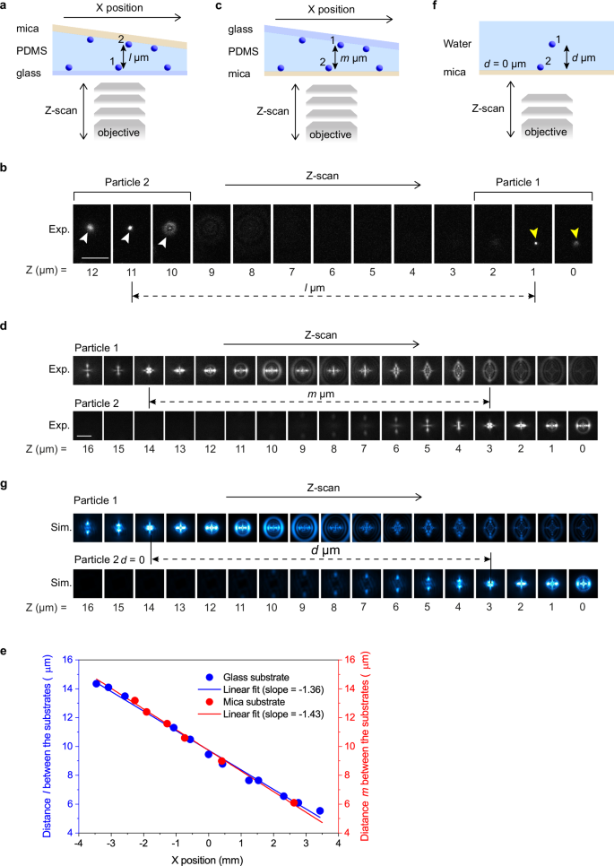
a A schematic illustration of the experimental configurations. 60 nm fluorescent nanospheres deposited on the glass and mica substrates were embedded in a wedge-shaped thin film of polydimethylsiloxane (PDMS). This experiment was conducted using a 164 µm-thick mica substrate. Fluorescence images were captured through the glass substrate. b Representative images of the fluorescent nanospheres deposited on the mica surface (Particle 2 indicated by white arrowheads) and the glass surface (Particle 1 indicated by yellow arrowheads) captured at varied Z-axis positions. Scale bar = 5 µm. c A schematic illustration of the experimental configurations. The experimental configurations were identical to those in (a), except that fluorescence images were captured through the mica substrate. d Representative images of the fluorescent nanospheres deposited on the glass surface (Particle 1) and the mica surface (Particle 2) captured at varied Z-axis positions. Scale bar = 5 µm. e The gap distances between the nanospheres deposited on the mica and glass surfaces determined at different X positions. The gap distances were determined by capturing the images through the glass (blue) and mica (red) substrates. The solid lines show linear fits. Two sets of samples were prepared and tested to ensure data reproducibility. f A schematic illustration of the configurations for the PSF simulation. A point emitter is placed either on the surface of a 164 µm-thick mica substrate or in the water at a distance from the mica surface of d µm. g Simulated PSF of the point emitter placed on the mica surface (Particle 2) and in the water at a distance from the mica surface of d µm (Particle 1) at varied Z-axis positions.
The PSF simulation conducted under similar conditions (i.e., PSF simulation for the emitters located on the surface of the mica substrate and located d μm above the surface, Fig. 5f, g) reproduced the experimentally observed PSF (Fig. 5d), also confirming the negligible impact of the mica to emitter distance on the PSF formation through the mica substrates. Our simulation showed that the PSF formed through a 185 μm-thick mica substrate is not affected significantly by the substrate-to-emitter distance of at least up to 20 μm (Supplementary Fig. 10). A slight change in the PSF becomes visible at longer substrate-to-emitter distances, particularly at the substrate-to-emitter distance of 30 μm (Supplementary Fig. 10). The simulation also indicates that a refractive index matching between the medium surrounding the emitter and the immersion medium minimizes the substrate-to-emitter distance-dependent change in the PSF (Supplementary Fig. 11).
Next, we performed a 3D localization experiment of fluorescent nanoparticles using the same wedge-shaped sample with different pre-defined Z-axis positions (Fig. 6a, b and Supplementary Fig. 12). The axial positions of the nanoparticles determined by the 3D localization at different pre-defined Z-axis positions are shown in Fig. 6c. The plots obtained from all the nanoparticles were fitted nicely to a linear function with slopes of 0.97–1.01(r2 = 0.99927–0.9999, Fig. 5j). This result demonstrates that the formation of the PSF pattern is unique to its axial position regardless of the emitter to mica distance, and the 3D localization accuracies of the emitters are not affected by their axial positions with respect to the mica surface.
Fig. 6: Effect of the emitter-to-mica substrate distance on the axial position localization.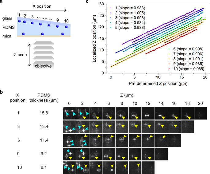
a A schematic illustration of the experimental configurations. The sample configurations were identical to those in Fig. 5c. b Representative Z-axis position-dependent images of the fluorescent nanospheres deposited on both surfaces captured at ten different X positions. The fluorescence images obtained for the nanospheres deposited on the glass and mica surfaces are indicated by yellow and cyan arrowheads. c Localized Z-axis positions of the fluorescence nanospheres deposited on the glass substrate at pre-defined focal positions of the microscope objective determined at ten different X-positions. The solid lines show linear fits. The data are plotted with an offset for clarity. Two sets of samples were prepared and tested to ensure data reproducibility.
Long-range 3D tracking measurements and diffusion tracking
We tested the effective axial range of our 3D tracking method by localizing and tracking multiple freely diffusing 60 nm fluorescent polystyrene nanoparticles distributed across a wide depth range in a homogeneous solution (glycerol-water 4:1 mixture) (Fig. 7a and Supplementary Movie 1). Freely diffusing nanoparticles in the sealed chamber (Fig. 7a) located at different axial positions are captured in the time-lapse images shown in Fig. 7b (denoted by green, cyan, and red arrowheads). These nanoparticles were successfully localized in 3D space, generating 3D diffusion time trajectories displayed in Fig. 7c. Notably, the diffusion trajectories distribute across the axial range of 30 µm (Fig. 7c). This demonstrates the capability of our 3D tracking method to track fluorescence emitters with an axial range of at least 30 µm, which is 50% wider than 20 µm, the previously reported maximum localizable depth range with the PSF engineering methods19.
Fig. 7: Quantitative analysis of diffusional motion using the birefringence-based single-particle 3D tracking.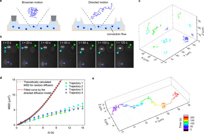
a Schematic illustrations of the sample configurations for the measurement of random diffusion using a sealed chamber (left) and directed diffusion using convection flow in an open chamber (right). This experiment was conducted using a 173 µm-thick mica substrate. b Representative time-lapse images of the 60 nm fluorescence nanoparticles freely diffusing in the sealed chamber. Three particles in the field of view are indicated by green, cyan, and blue arrowheads. The images were captured at a 1 Hz repetition rate with 100 ms exposure time. c Localized 3D diffusion trajectories of the three fluorescent nanospheres obtained from the time-lapse images in (b). d Mean square displacement (MSD) versus time lag plots obtained from the diffusion trajectories shown in (c) and (e). The dashed line shows the theoretically calculated MSD versus time lag plot of the nanospheres in a medium with 1 mPa s viscosity using the diffusion constant of the fluorescent nanospheres estimated by Eq. 7. The solid line shows fitting to the directed diffusion model (Eq. 6). Four sets of samples were prepared and tested to ensure data reproducibility. e Localized 3D diffusion trajectory of a fluorescent nanosphere obtained using the open chamber.
The applicability of our 3D tracking method to the quantitative characterization of diffusional motions was examined by mean square displacement analysis. Using the 3D diffusion trajectories (Fig. 7c) obtained in the sealed chamber, we calculated MSD versus time-lag plots for each trajectory (Fig. 7d). The MSD versus time lag plots can be fitted to a linear function (i.e., random diffusion, Fig. 7d). The diffusion constant (D) of the nanoparticles was estimated to be 0.0744 µm2 s-1, calculated from the slope of the averaged MSD plot obtained from the three localized trajectories (Supplementary Fig. 13). This value agrees with the D value calculated by the Einstein-Stokes equation (D = 0.0783 µm2 s-1; see Methods for the details)39,40. The simulated MSD versus time lag plot with this calculated D value also agrees with the experimentally obtained MS plots (Fig. 7d). The linear MSD plot, together with the excellent agreement between the experimentally obtained and simulated MSD, indicate that our 3D tracking method can be used for the quantitative characterization of the 3D motion of the fluorescent nanoparticles. The MSD plot obtained from Trajectory 3 in Fig. 6c slightly deviates from a linear function (Fig. 7d), which could be attributed to the physical interaction between the nanoparticle and the mica surface.
Figure 7e shows a representative 3D diffusion trajectory of the nanoparticles captured in the open chamber (Fig. 7a and Supplementary Movie 2), where the directed diffusion caused by convection flow is clearly seen. The MSD versus time lag plot obtained from the diffusion trajectory (Fig. 7d) was fitted to the directed diffusion model, from which the diffusion constant (D = 0.0885 µm2 s-1) and flow velocity (v = 0.305 µm s-1) were estimated. The estimated D value is similar to that obtained for the random diffusion. The result also suggests the applicability of our 3D tracking method for the quantitative characterization of the 3D motion of the fluorescent nanoparticles.
Notably, we could record 3D diffusion trajectories over the 3500 image frames for over 11 min (Supplementary Fig. 14). This was possible because of the small PSF in the extended axial range, which allowed us to capture the fluorescence images with a high signal-to-background ratio at the reduced excitation power range, minimizing the photobleaching effect over the extended period of time.
3D tracking in plant cells
The applicability of our method to the 3D tracking in a biological sample was evaluated using live cells. We first applied our 3D tracking method to mammalian cells (see Methods for details of the sample preparation). As shown in Supplementary Fig. 15, 3D diffusion trajectories of the fluorescent nanospheres deposited on Chinese hamster ovary cells were tracked using our method, demonstrating the applicability of our method to 3D tracking in mammalian cells. Next, we applied our method to plant cells (Fig. 8a). Plant cells represent unique challenges for fluorescence microscopy, especially for single-particle 3D tracking, due to high autofluorescence, significant refractive index mismatches within cell structures (e.g., between the cytoplasm and cell wall), and their large size. Previously reported 3D tracking techniques have never been applied to tracking experiments in plant cells, partly due to these challenges. Using 3.5 nm size organic J-aggregate nanoparticles that emit bright fluorescence41, we conducted a 3D tracking experiment in onion (Allium cepa L.) epidermal cells, whose size is approximately 200 µm (length) × 50 µm (width) × 40 µm (height) (Fig. 8b and Supplementary Movie 3, see Methods for details of the sample preparation). Each image was recorded with a short exposure time of 6 ms and a time interval between the images of 30 ms to obtain sharp images of the rapidly moving nanoparticles (see Methods for experimental details). Bright-field images of the same sample region were also recorded (Fig. 8c). Notably, the mica substrate had a negligible effect on the quality of bright-field images (Fig. 8c). The time-lapse images obtained from a single fluorescent nanoparticle injected into the cells show that the fluorescence image of the nanoparticle and the time-dependent changes in its spatial pattern are clearly captured (Fig. 8b). We were able to capture more than 1500 frames of images of the tracked nanoparticle, from which we obtained the 3D diffusion trajectory of the nanoparticle in the plant cell (Fig. 8d). The result suggests that our 3D tracking method is applicable to biological samples, including challenging specimens for optical microscopy, such as plant cells.
Fig. 8: Birefringence-based single-particle 3D tracking in plant cells.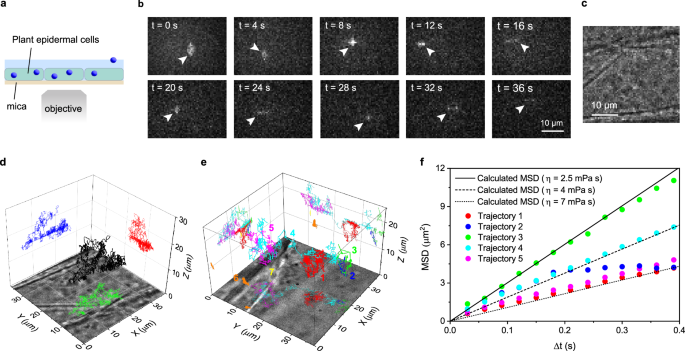
a A schematic illustration of the sample configurations for the 3D tracking experiment in plant cells. This experiment was conducted using a 170 µm-thick mica substrate. b Representative time-lapse fluorescent images of 3.5 nm size fluorescent nanoparticles injected into the plant cells. A particle in the field of view is indicated by arrowheads. c A bright-field transmitted microscopy image captured at the same sample position as the fluorescence imaging experiment shown in (b). d Localized 3D diffusion trajectory of a fluorescent nanoparticle in the cell obtained from the time-lapse images in (b). e Localized 3D diffusion trajectories of multiple fluorescent nanoparticles inside the cell. f Mean square displacement (MSD) versus time lag plots obtained from the five diffusion trajectories shown in (e). The solid, dashed, and dotted lines show the theoretically calculated MSD versus time lag plots of the nanoparticles in a medium with 2.5, 4, and 7 mPa·s viscosity using the diffusion constant of the fluorescent nanoparticles estimated by Eq. 7. Three sets of samples were prepared and tested to ensure data reproducibility.
Figure 8e shows an example of the 3D tracking of multiple fluorescence nanoparticles located at different axial positions in a plant cell. Seven trajectories distributed over a 20 µm axial range inside the cell were localized, demonstrating the multiplexing capability and large axial range of our 3D tracking method (Supplementary Note 6). The five nanoparticles (denoted by 1, 2, 3, 4, and 5 in Fig. 8e) exhibited 3D diffusional motion in the cell, and we characterized their motion by the MSD analysis (Fig. 8f). Two other nanoparticles (denoted by 6 and 7 in Fig. 8e) in the cell showed negligible motion throughout the imaging experiment, most likely due to anchoring to an inner surface of the cell. The MSD versus time lag plots obtained from these nanoparticles clearly show different slopes (i.e., distinct diffusion rates) and curvatures (i.e., distinct diffusion modes). While the MSD versus time lag plots obtained from trajectories 1, 3, 4, and 5 agree very well with the simulated MSD plot assuming a random diffusion of the particle in a homogenous medium with its viscosity slightly higher than that of water (2.5, 4, and 7 mPa s for trajectory 5, trajectory 4, and trajectories 1 and 3, respectively), the MSD plot obtained from trajectory 2 deviates significantly from the simulated random diffusion. These results demonstrate that our 3D tracking method can be used for the quantitative characterization of the velocity and modes of the motion of individual nanoparticles in biological samples, including plant cells.