
Sign up for the Starts With a Bang newsletter
Travel the universe with Dr. Ethan Siegel as he answers the biggest questions of all.
In many ways, the Big Bang was the biggest idea to ever come out of Einstein’s General theory of Relativity. This tremendously successful theory gave us everything from gravitational waves to black holes based on one profound insight: that the fabric of spacetime itself would evolve, curve, and even ripple based on the properties and behavior of the matter and energy within it. When we applied Einstein’s equations to the entire Universe as a whole, along with the idea that the Universe was filled nearly uniformly with matter and energy on the largest scales, we wound up with an expanding Universe. Extrapolating back in time, we arrived at a very hot, dense, and uniform early state, where all of the Universe’s matter and energy was concentrated into a tiny, minuscule volume.
And yet, if we look at the evidence that persists in the Universe today, left over from those early cosmic stages, we find that the hot Big Bang couldn’t have risen all the way up to the hottest possible temperatures: temperatures corresponding to the Planck scale. Those high energies, corresponding to around 1019 GeV or 1032 K, would have imprinted signatures in the cosmic microwave background (CMB) that simply aren’t present. Instead, the signatures that do show up in the CMB tell a very different tale: one of an inflationary past that was then followed by a much “less hot” early, dense, expanding state.
We still don’t know how hot the Big Bang was in its hottest, earliest stages, but we do have both upper and lower limits that guide our quest for further knowledge about our cosmic beginnings.
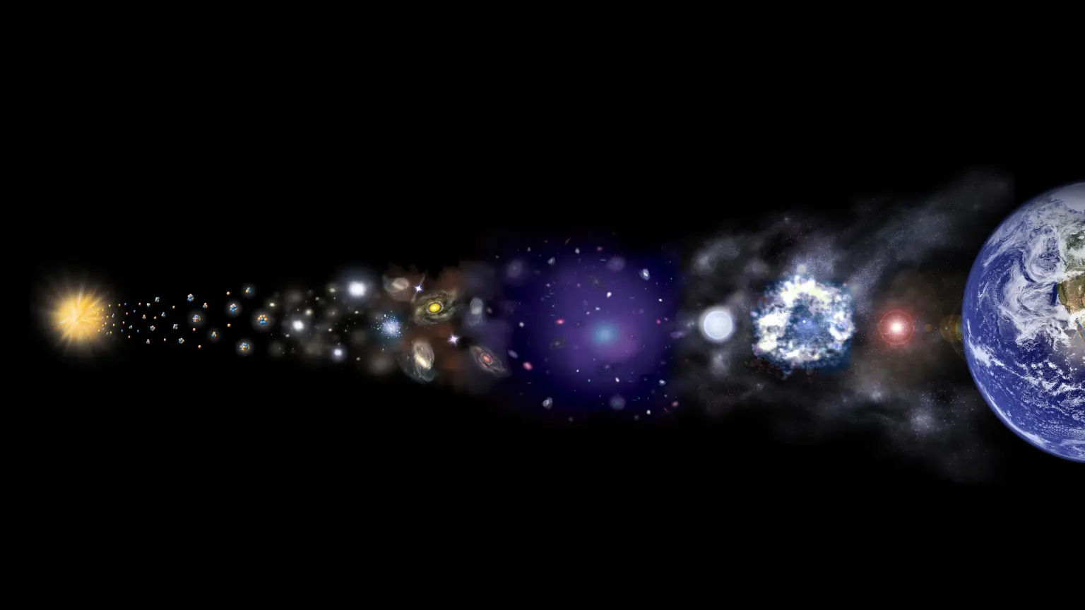
Our Universe, from the hot Big Bang until the present day, underwent a huge amount of growth and evolution, and continues to do so. Our entire observable Universe was approximately the size of a modest boulder some 13.8 billion years ago, but it has expanded to be ~46 billion light-years in radius today. The complex structure that has arisen must have grown from seed imperfections of at least ~0.003% of the average density early on, and has gone through phases where atomic nuclei, neutral atoms, and stars first formed, eventually giving rise to our Solar System, planet, life, and humans.
Credit: NASA/CXC/M. Weiss
The story of the Big Bang began back in the 1920s, when two important parallel developments occurred. On the theoretical side, Alexander Friedmann took Einstein’s field equations and considered what would happen if the Universe were uniformly filled with any form of energy at all. He found that there was no static, stable solution that was possible, save if the Universe were entirely empty. If there was anything in your Universe at all, it must either expand or contract, with the equations that he derived — the Friedmann equations — detailing how the rate of cosmic expansion (or contraction) and its evolution would relate to the energy contents of the Universe.
Also in the 1920s, Edwin Hubble, along with his assistant Milton Humason, began observing individual stars in galaxies beyond the Milky Way, enabling us to measure the distances to these nebulous objects. Combined with Vesto Slipher’s earlier observations of the redshifts (or, occasionally, blueshifts) of those galaxies, we found that the more distant a galaxy was from us, the faster it appeared to be receding. This was consistent with the idea that the Universe was expanding.
Putting these two pieces of theoretical and observational work together allowed us to conclude that yes, the Universe was expanding. As time went on, we measured just how fast it was expanding, with better data from the Universe’s past showing us the expansion rate’s evolution: allowing us to infer what the contents of the Universe itself are.
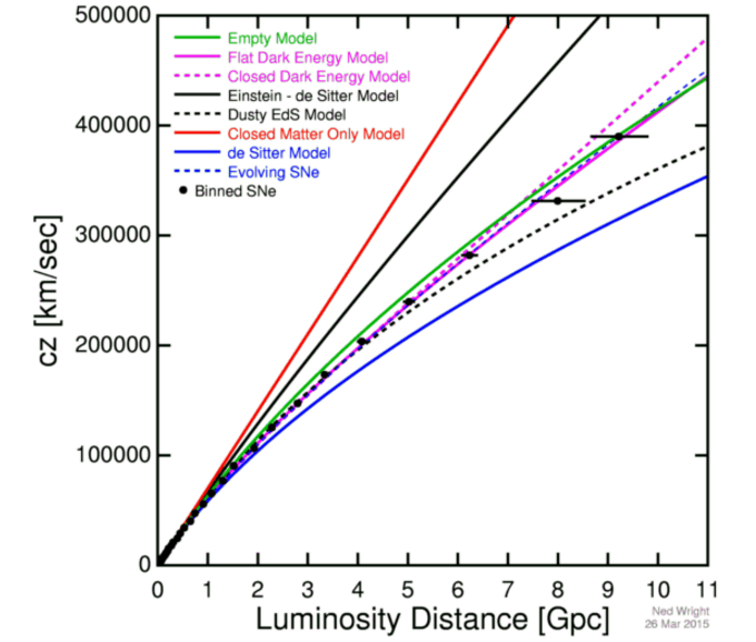
A plot of the apparent expansion rate (y-axis) vs. distance (x-axis) is consistent with a Universe that expanded faster in the past, but where distant galaxies are accelerating in their recession today. This is a modern version of, extending thousands of times farther than, Hubble’s original work. Note the fact that the points do not form a straight line, indicating the expansion rate’s change over time. The fact that the Universe follows the curve it does is indicative of the presence, and late-time dominance, of dark energy.
Credit: Ned Wright/Betoule et al. (2014)
Once nice thing about Friedmann’s equations is how deterministic they are. If you know what the Universe is made of and how fast it’s expanding at any point in time, you can compute all sorts of properties about our cosmic past. With the mix of dark energy, dark matter, normal matter, neutrinos, and photons that we have in our Universe today, coupled with the measured expansion rate, we can conclude that our Universe has been around for 13.8 billion years, was dominated by radiation early on, and did indeed have a hot, dense, very uniform past. In fact, if we look today, we can see the leftover photon glow from that early stage: that’s what the CMB is.
When we look at the properties of the CMB in detail, we find some remarkable pieces of information inside.
It confirms our picture of a Universe that’s spatially very flat, without significant positive or negative curvature.
It shows us a Universe that’s incredibly uniform: with the same temperature of 2.7255 K everywhere and in all directions.
It exhibits tiny, few-parts-in-100,000 temperature fluctuations, which are Gaussian (random variable) in nature and are almost scale-invariant: about 3% larger in magnitude on large scales than small scales.
It reveals a Universe with both dark matter and normal matter, where dark matter outmasses normal matter by approximately a 5-to-1 ratio.
And it shows us temperature fluctuations that are polarized as well: with both (E-mode and B-mode) types of polarizations present.
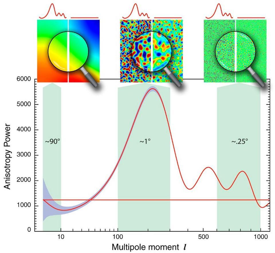
The fluctuations in the cosmic microwave background, as measured by COBE (on large scales), WMAP (on intermediate scales), and Planck (on small scales), are all consistent with not only arising from a (slightly tilted, but almost-perfectly) scale-invariant set of quantum fluctuations, but of being so low in magnitude that they could not possibly have arisen from an arbitrarily hot, dense state. The horizontal line represents the initial spectrum of fluctuations (from inflation), while the wiggly one represents how gravity and radiation/matter interactions have shaped the expanding Universe in the early stages.
Credit: NASA/WMAP science team
This light, when we first detected it, was hailed as the “smoking gun” proof that the Big Bang occurred. This leftover glow, among its other properties, exhibited a blackbody spectrum: precisely the spectrum (i.e., energy distribution) that we’d expect if it was of primeval, cosmic origin. However, puzzles with the hot Big Bang — of things we observed but that the Big Bang with an arbitrarily hot, dense past couldn’t explain — were swiftly pointed out by people like Bob Dicke and Jim Peebles. These puzzles, like the horizon problem, the flatness problem, and the monopole problem, strongly suggested that the hot, dense, early state couldn’t be extrapolated to arbitrarily high temperatures and energies.
The solution was proposed back in 1980/1981: a period of cosmic inflation (relentless, exponential expansion that had a form of energy inherent to space itself, rather than matter or radiation, dominating the Universe) that set up and preceded the hot Big Bang. Not only would inflation solve these three puzzles, as it would:
give the observable Universe the same properties everywhere, having inflated them from a tiny region that had the same properties throughout it,
stretch the Universe to be indistinguishable from perfectly flat, regardless of its prior properties,
and “only” heat the Universe up to some sub-Planckian maximum temperature, avoiding the creation of monopoles and other pathological relics,
but it would also lead to a series of novel predictions that would differ from the non-inflationary hot Big Bang that did reach arbitrarily high (e.g., Planck-like) temperatures.
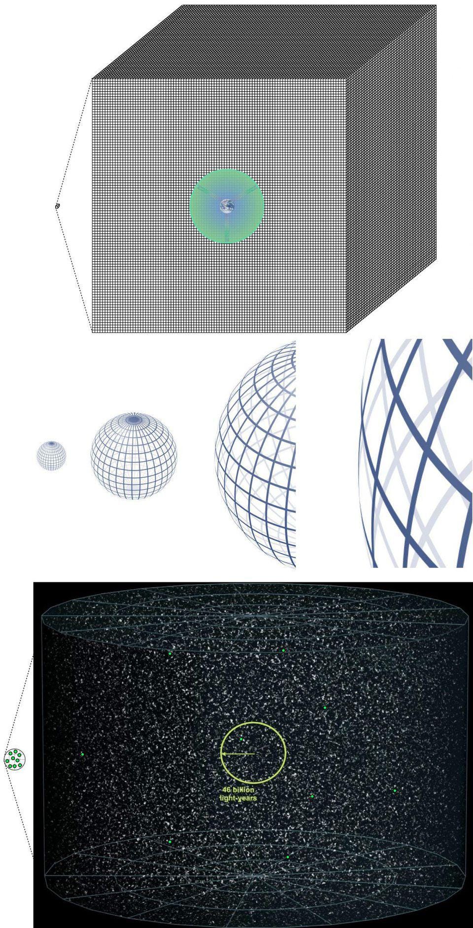
In the top panel, our modern Universe has the same properties (including temperature) everywhere because they originated from a region possessing the same properties. In the middle panel, the space that could have had any arbitrary curvature is inflated to the point where we cannot observe any curvature today, solving the flatness problem. And in the bottom panel, pre-existing high-energy relics are inflated away, providing a solution to the high-energy relic problem. This is how inflation solves the three great puzzles that the Big Bang cannot account for on its own.
Credit: E. Siegel/Beyond the Galaxy
What those new predictions would be fell into two categories:
predictions that would be rather generic under the conditions of inflation, irrespective of what particular “flavor” of inflation occurred (i.e., that were roughly model-independent),
and predictions that would be highly dependent on either the specific model of inflation being considered or the particular properties that inflation possessed.
Generic predictions include the same initial temperature everywhere, with a spectrum of seed fluctuations imprinted atop it that are Gaussian in nature and almost, but not quite, identical across cosmic scales. Those fluctuations should be 100% adiabatic (of constant entropy) and not isocurvature (of the same spatial curvature) in nature. The post-inflationary Universe should be very close to spatially flat, but with small imperfections on the scale of 0.0001% to 0.01%. And it should produce a spectrum of gravitational wave fluctuations as well: of specific relative magnitudes on a variety of scales.
But how would that spectrum of seed fluctuations differ from perfect scale-invariance?
What would the amplitude of those gravitational wave fluctuations be?
And how hot would the Universe have gotten, at maximum, once inflation came to an end and the Universe became filled with matter and radiation, signifying the start of the hot Big Bang?
These questions, among others, are prominently model-dependent. To approach answering them, we need a way of distinguishing between the different “flavors” of inflation.
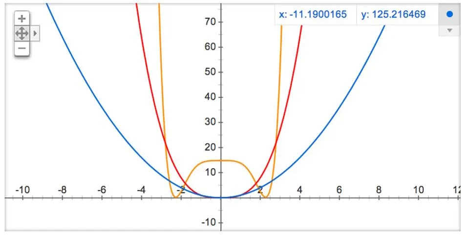
Three possible ‘hills-and-valleys’ potentials that could describe cosmic inflation. Though they give somewhat different results for the various parameters of the Universe, there is no motivation, save for the constraints on parameters like the maximum reheat temperature, the scalar spectral index and its running, and the r-ratio for tensor-to-scalar fluctuations, when it comes to preferring any one particular inflationary model over another.
Credit: E. Siegel/Google Graph
What you see, above, are a few examples of what we call “potentials” in theoretical physics. A potential is any one-dimensional line, two-dimensional surface, or more complicated (and possibly higher-dimensional) structure where you can imagine:
dropping down a ball anywhere on it,
that ball will naturally roll down, at some speed, to some local minimum,
and will either remain there or continue on, either through rolling or through quantum tunneling, until it reaches the “true” minimum of the potential.
For the red and blue curves above, that minimum is at “0” on the x-axis, while for the yellow curve, there are two minima: one on the positive side and one on the negative side.
Although you can easily concoct a more complicated inflationary model than the examples illustrated above — multidimensional models, multi-field models, vector or tensor models (instead of just the scalar model shown here), etc. — it is neither necessary nor particularly helpful to do so. Nearly all of the phenomena that vary between models can be encapsulated by either a simple one-dimensional scalar potential, as shown, or by an “effective potential” that is, for all practical purposes, identical to a one-dimensional line like this.
However, the particular properties of the line you draw can lead to vastly different observables.
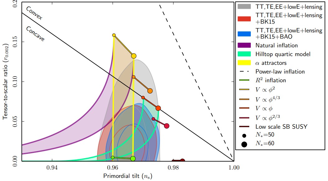
Various models of inflation and what they predict for the scalar (x-axis) and tensor (y-axis) fluctuations from inflation. Note how just a small subset of viable inflationary models gives rise to a huge variety of possible predictions for these parameters, and how even with the joint constraints provided by various independent cosmological probes, that many models of inflation remain viable and consistent with the data.
Credit: Planck collaboration, Astronomy & Astrophysics, 2020
For example, take a look at the graph above. What you can see there are different possible values for two of the measurable parameters:
the scalar spectral index (or the primordial tilt), denoted by the parameter ns,
and the tensor-to-scalar ratio, sometimes denoted by the parameter r,
where different points and colors correspond to different inflationary potentials and different numbers of what we call “e-foldings” (or how many times the Universe expanded by a factor of the number e) during the period of cosmic inflation.
On the other hand, the contours correspond to (2018-era) constraints on both of those parameters: ns and r. Different potentials that you can draw will lead to different values for these parameters, where generically the U-shaped potentials have large r values and the plateau-like potentials have smaller ones. They can also take on different values for ns, where both the U-shaped and plateau-like potentials have values that are slightly less than 1, whereas hybrid models (or two-field models) of inflation typically yield values for ns that are slightly greater than 1. Because of our observations that we’ve made, we can rule those classes of inflation out, while the U-shaped models are more tightly constrained by B-mode polarization measurements.
The contribution of gravitational waves left over from inflation to the B-mode polarization of the cosmic microwave background has a known shape, but its amplitude is dependent on the specific model of inflation and can only be constrained observationally. These B-modes from gravitational waves from inflation have not yet been observed, but detecting them would help us tremendously in pinning down precisely what type of inflation occurred. A false detection, from the BICEP2 team, famously occurred in the early 2010s, but was swiftly refuted. We now know that the r-ratio, represented on the y-axis, must be no greater than about ~0.01, with future experiments hoping to get down to the 0.001 or even the 0.0001 level.
Credit: Planck Science Team
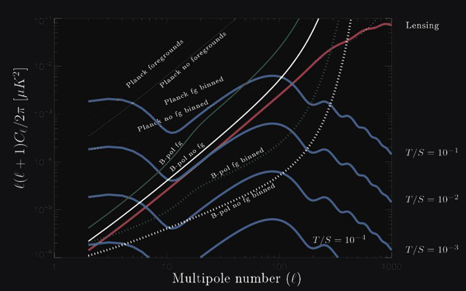
Looking at those B-mode polarization predictions, in detail, can also shed a lot of light on how well (or poorly) inflation can be constrained by our current and upcoming near-future observations.
What you see, above, is an example of the gravitational wave spectrum predicted by inflation, and in particular, how that spectrum imprints itself on the B-mode polarization of the CMB. The blue lines, from top-to-bottom, indicate the inflationary contribution to that B-mode polarization, but for different models: in particular, for models that predict different tensor-to-scalar ratios, sometimes called r-ratios. If you have a keen eye, you might notice that those blue lines are all identical in terms of the patterns of peaks-and-wiggles that the curves possess; only the amplitude differs.
There’s a good reason for this: the inflationary properties that produce the primordial gravitational wave spectrum do not vary significantly between inflationary models in terms of what fluctuations will appear on which scales. What varies, instead, is the height, or amplitude (or magnitude) of those fluctuations.
If you’re curious, that might lead you to ask a key question: what causes those variations? Similarly, for the scalar spectral index, ns, as well as its running, as well as a few other properties (like the maximum temperature achieved when inflation ends and the hot Big Bang begins) that vary from model-to-model, you might ask what causes all of the variations that exist between inflationary models?
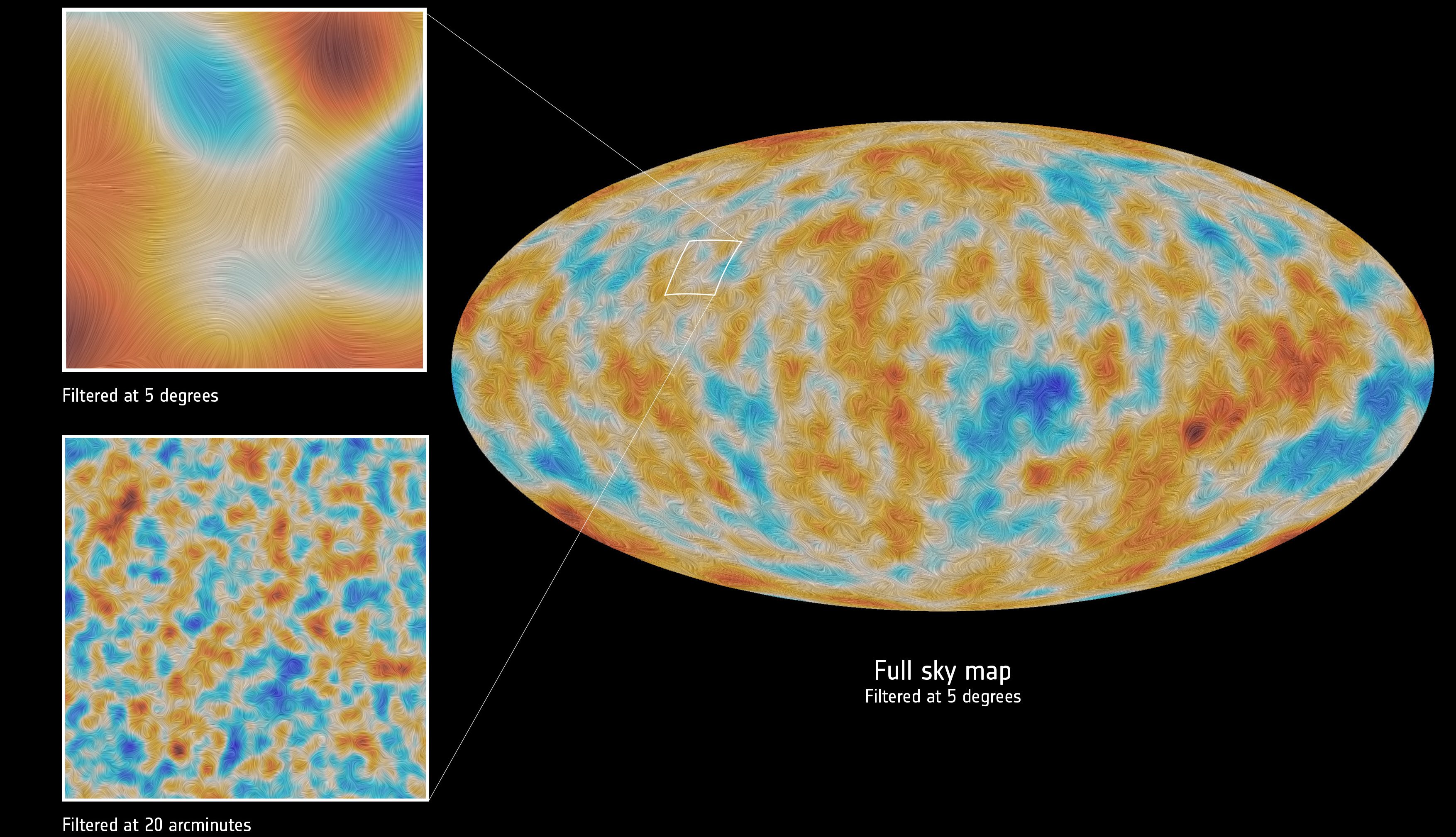
This map shows the CMB’s polarization signal, as measured by the Planck satellite in 2015. The top and bottom insets show the difference between filtering the data on particular angular scales of 5 degrees and 1/3 of a degree, respectively. While temperature data, alone, can demonstrate that the CMB is of cosmic nature, the polarization signal gives us key pieces of information relevant to the details of cosmic inflation.
Credit: ESA and the Planck Collaboration, 2015
As it turns out, there are only three things that are generally relevant.
What is the height of the potential, or the y-axis value of the curve that describes inflation, during the final ~60 or so e-foldings of inflation?
What is the derivative, or the slope, of the potential during those same critical final 60-or-so e-foldings of inflation?
And what is the second derivative, or the concavity, of the potential during those same relevant e-foldings of inflation?
That’s it. You calculate those three properties of any candidate inflationary potentials that you like, you apply the results appropriately, and you can then go and predict what sorts of observables your inflationary model would lead to. You can also compare how those values fare when confronted with the data we already have.
And we have lots of data: data from the cosmic microwave background, data from the large-scale structure observed throughout the Universe and across cosmic time, data about our cosmic expansion rate throughout history, and even data from cosmic rays about the maximum energies that particles achieve, and hence, about energies that particles reach when they collide with one another.
From the full suite of data, we can conclude that the maximum temperature the Universe could have reached after the end of inflation is around 1028 K (1015 GeV), and also that the maximum energy that cosmic rays collide at today is no greater than about 1010 GeV in energy, or a corresponding temperature of 1023 K.
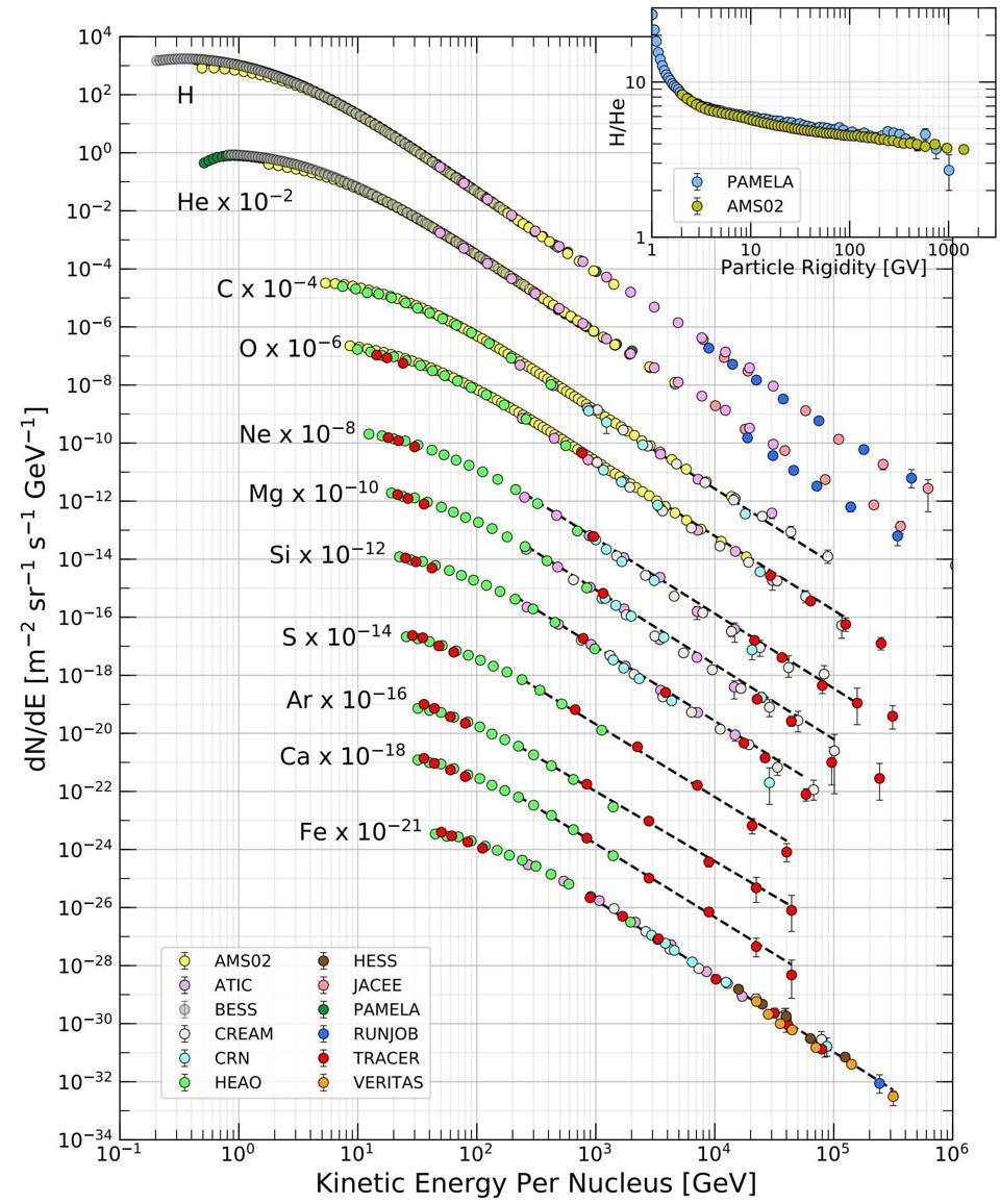
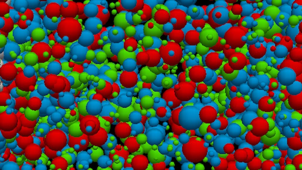
Cosmic ray spectrum of the various atomic nuclei found among them. Of all the cosmic rays that exist, 99% of them are atomic nuclei. Of the atomic nuclei, approximately 90% are hydrogen, 9% are helium, and ~1%, combined, is everything else. Iron, a low-abundance but important example of the heavy, high-energy atomic nuclei found, may compose the highest-energy cosmic rays of all: found with up to 10^11 GeV of energy.
Credit: M. Tanabashi et al. (Particle Data Group), Phys. Rev. D, 2019
Although there is wiggle-room for the inflationary temperature/energy scale to be a bit lower than the limit set by cosmic rays, the CMB limits on the maximum post-inflationary temperature cannot be evaded. This has extremely important implications for what the r-ratio (the tensor-to-scalar ratio) of the gravitational waves produced by inflation would be. For every factor of 10 lower in energy, the tensor amplitude drops by a factor of 10,000, as it scales as the value on the y-axis (the energy density value) to the fourth power.
This is, to be blunt, a huge effect!
There are people who are dedicating their scientific (and in some cases, their entire) lives to the search for B-mode polarization signals in the CMB — the only way that we know that such a gravitational wave signal from inflation would manifest itself — and we have to be careful to remember the old adage that “absence of evidence is not evidence of absence.” While detecting the characteristic signature from these gravitational waves would be revolutionary, there’s no guarantee that’s possible. A plateau-like inflationary potential at around 1015 GeV would lead to an r-ratio of 0.0001 or greater, but a potential at only around 1011 GeV would have an r-ratio that’s unmeasurably small: around 10-20. If the cosmic ray bound turns out to be meaningless, r is allowed to be even lower.
And yet, this substantial space of uncertainty gives us a relatively narrow range for the maximum temperature of the Universe, after the end of inflation, at the start of the hot Big Bang: between 1024 and 1028 K. This is at least a factor of a few thousand below the Planck scale, but tens of millions of times greater than the maximum energies achievable at the Large Hadron Collider. There’s a lot we still don’t know about the origin of the Universe, but as I said not so long ago:
“our observations can constrain parameter space to the limits that they can constrain it to. That is neither feature nor bug; that is a fact of any experimental/observational science.”
Sign up for the Starts With a Bang newsletter
Travel the universe with Dr. Ethan Siegel as he answers the biggest questions of all.