
Mapping recognized Afro-descendant lands
We first collated and combined spatial datasets delineating ADP lands with legal tenure recognition. In the context of this paper, we use ADP lands, recognized ADP lands and recognized Afro-descendant lands interchangeably; all refer to delineated areas in which ADP communities possess recognized tenure (at minimum management rights). We considered ADP to have management rights if they can make decisions about their lands and resources within those lands.
We collected legal tenure information through which ADP land rights are recognized in each study country. We identified the legislation that first recognized the tenure system and rights of Afro-descendant communities to lands and waters and the years enacted, as well as the bundle of rights (access, use, management, exclusion, alienation) conferred to the communities through legislation, for each country (Supplementary Table 1). Legislation information was obtained primarily from FAOLEX80,81,82,83. Secondary supporting documents, such as peer-reviewed papers or NGO reports clarifying nuances or to better understand the legal frameworks and history of rights conferred, were obtained from other sources. ADP may also have other property rights described in the bundle of rights concept84.
Our study area covers four South American countries (Brazil, Colombia, Ecuador, and Suriname) where ADP communities have legally recognized land tenure rights to communal governance and management of their lands, and where we could obtain spatial datasets. In these countries, except for Suriname, ADP communities not only have legally recognized rights to manage lands but also possess or are in the process of receiving (such as in the case of certain quilombos in Brazil) collective titles through which they communally own delineated territories. In Suriname, ADP lack full legally recognized rights and thus are unable to obtain territorial ownership through collective titling or other means. However, we include ADP lands in Suriname in this study because we consider ADP in Suriname to at least have partial legally recognized tenure: through the Forest Management Act of 1992 (Wet Bosbeheer 1992, No. 80), they can have management rights to community forestry concessions for logging and customary land surrounding their villages. Recognized ADP lands in Suriname in our study represent areas that we could determine these management rights apply.
We obtained the recognized ADP lands datasets from the governmental web portals of Instituto Brasileiro de Geografia e Estatística (IBGE)85 for Brazil and Agencia National de Tierras (ANT)86 for Colombia; from EcoCiencia for Ecuador87; and from Conservation International for Suriname, which co-mapped spatial datasets in collaboration with and in support of the Matawai community (Supplementary Table 1). Country boundary polygons for all study countries were obtained from Global Administrative Areas (GADM) (version 4.1, 2022)88 and Esri89. Administrative unit boundary polygons were obtained from IBGE90 for Brazil, from Departamento Administrativo Nacional de Estadística (DANE)91 for Colombia, and from GADM (version 4.1, 2022)88 for Ecuador and Suriname.
Calculating the extent of ADP lands
To calculate areas of ADP lands, we used the ArcGIS Pro Python site package ‘ArcPy’ to automate spatial data processing and ensure that the ADP tenure spatial datasets would be uniformly processed. All ADP lands datasets were processed in ArcGIS Pro (version 3.2) and projected to WGS 1984 Web Mercator Auxiliary Sphere (WKID 3857) to maximize utility in calculating area numbers, determining areas of overlap across platforms, and overlaying other datasets. For consistency, all area values were then calculated using R Studio or Google Earth Engine (GEE).
There are limitations inherent to spatial analyses, which may occur due to approaches used to quantify the extent and presence of ADP lands. Limitations may be caused by different levels of accuracy for each input ADP lands dataset depending on how datasets were mapped by their creators, by the need to standardize ADP lands datasets to one coordinate system from different initial coordinate systems, and by differences between software and platforms used for processing and analysis (ArcGIS Pro, R, GEE). These limitations may also apply to other input datasets used.
The extent of recognized ADP lands we calculated does not reflect the extent of customary or ancestral territories of ADPs, much of which remains unrecognized. As such, our study only shows a conservative estimate of the extent of ADP lands in the four countries we examined, whereas ADP presence in other countries of the Americas and the Caribbean is documented elsewhere9,92. Further limitations to mapping the extent and presence are detailed in the Supplementary Note 1 section of this paper.
Mapping Afro-descendant presence
Information on the number and percentage of self-identified Afro-descendants in Brazil, Colombia, Ecuador, and Suriname (Supplementary Tables 3, 4) were derived from tabular datasets containing demographic information within level-2 administrative units from each country’s most recent census93,94,95,96. For Brazil and Colombia, Afro-descendant presence specifically within ADP lands, in addition to per administrative unit, was included as a component of population data for both censuses. For Ecuador and Suriname, since Afro-descendant presence was only included per administrative unit, we determined which administrative units overlap ADP lands by intersecting administrative unit88 and ADP land data we obtained for both countries. The Afro-descendant presence map (Supplementary Fig. 1) was created by joining census data with level-2 administrative unit data for each country (see administrative unit data sources in the Data Availability section below)88,90,91.
ADP lands, ecosystems, and protected areas
To provide additional context about the locations of ADP lands, we calculated the extent to which ADP lands overlap ecosystems and PAs within the study countries ArcGIS Pro (version 3.4). We determined which biomes and ecosystems overlap ADP territories in each country by projecting the RESOLVE Ecoregions and Biomes layer97 to WKID 3857, pairwise intersecting with the ADP territories layer, then calculating areas of overlap (ha). We determined which PAs overlap ADP territories by filtering the WDPA polygon layer98 by country (including Brazil, Colombia, Ecuador, and Suriname) and designation status (excluding Proposed), projecting to WKID 3857, pairwise intersecting with the ADP land layer, then calculating areas of overlap (ha). Since areas of overlap were determined through spatial analysis of polygon extents, we did not repeat this analysis for the WDPA points layer.
Calculating biodiversity within ADP lands
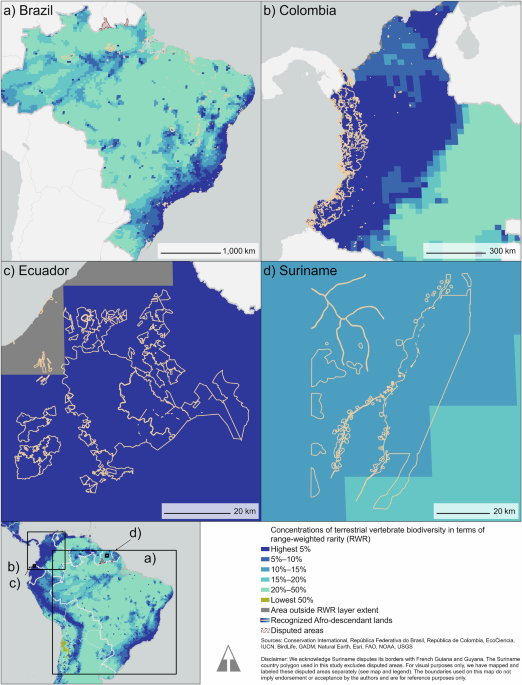
To estimate the spatial distribution of different levels of global importance for biodiversity in terms of terrestrial vertebrate species (amphibians, birds, mammals, and reptiles), we used a global RWR raster layer at 30-km resolution. This biodiversity metric shows the relative importance of a grid cell by accounting for both the number of species potentially present and the extent of their total ranges. The RWR raster, produced by IUCN using the Red List version 2023-1, represents where thousands of terrestrial vertebrate species are potentially present99,100,101. This metric is based on habitat ranges mapped by experts and informed by occurrence data, but values at a given point do not represent confirmed occurrences. Therefore, values represent the potential number of species present, given the overlap of geographic ranges with suitable habitat. The level of detail in the global database may not sufficiently capture local variations, and the accuracy of the database may vary by geographic region, as the quality of expert information could differ. These limitations have been captured by previous studies102.
Based on the global RWR raster, we estimated the spatial distribution of different levels of global biodiversity by calculating 5%, 10%, 15%, 20%, and 50% threshold values and masked the global raster to values at or above the corresponding thresholds. We clipped these masked global RWR rasters by the spatial extents of each region of interest (ROI): recognized ADP lands as well as overall areas nationally across the four study countries (Fig. 1). We then estimated how much of each ROI extent has high biodiversity by calculating the total number of pixels within each extent. The continent of Antarctica was removed from the global RWR raster before performing this analysis.
For additional biodiversity analysis, we evaluated the intersection of the spatial extent of each ROI with each species habitat range to generate lists of all terrestrial vertebrate species with ranges overlapping each ROI, as well as total species per taxonomic group (amphibians, birds, mammals, and reptiles) and IUCN Red List category (Critically Endangered, Endangered, Vulnerable, Lower Risk, Near Threatened, Least Concern, and Data Deficient)100,101. To account for ranges of certain species covering multiple countries in the study area, we analyzed each ROI individually within each country and across all study countries. With these output lists, for each ROI we determined the composition of terrestrial vertebrate species by their taxonomic groups and IUCN Red List categories and compared lists for all ROIs. All biodiversity spatial analysis was implemented in R statistical software version 4.3.1103, primarily through the’terra’ package version 1.7.39104.
Calculating irrecoverable carbon within ADP lands
We also intersected the spatial extent of each ROI with a global irrecoverable carbon20 raster to estimate total tonnes of irrecoverable carbon as well as generate lists of tonnes of irrecoverable carbon per ecosystem (mangroves, tropical and subtropical grasslands, tropical and subtropical forests, tropical and subtropical wetlands, and tropical peatlands). We generated these estimates for each ROI. We then calculated the proportion of irrecoverable carbon that is high irrecoverable carbon (>25 t/ha) following a previous publication20, and the average irrecoverable carbon (t/ha) within every ROI. Irrecoverable carbon values were generated using GEE.
We visualized levels of high irrecoverable carbon within recognized ADP lands and per country using the Irrecoverable Carbon 2018 dataset20 to map global irrecoverable carbon across ecosystems. We assigned the same irrecoverable carbon thresholds as the intersection analysis by a previous publication20 to the dataset’s pixel values, where areas containing high irrecoverable carbon have pixel values > 25 (t/ha).
The study by Noon et al. (2022) on mapping irrecoverable carbon does acknowledge certain limitations in quantifying irrecoverable carbon, including uncertainty in global estimates of irrecoverable carbon due to variability in data quality and availability across different ecosystems. This uncertainty can impact the precision of mapping. On smaller scales and at the pixel-level, this uncertainty falls within reasonable ranges; thus, we do not anticipate that this global uncertainty will significantly affect this study or the relative comparison of high irrecoverable carbon concentrations within ADP lands.
Quasi-experimental design and analysis: sampling grid
We subsampled areas inside and outside of ADP lands using a 300 m resolution sampling grid. This cell size was chosen to balance considerations of sample size, computation time, and spatial coverage of ADP lands (e.g., data exploration showed that larger cell sizes would exclude coverage of many smaller ADP polygons). To produce the sampling grid for statistical matching and quantifying forest cover change, we first overlaid ADP lands from Brazil, Colombia, Ecuador, and Suriname with country boundaries and removed island regions (Providencia Island, Colombia, and Galápagos Islands, Ecuador) that did not intersect with our spatial dataset of ADP lands. To generate treatment cells – i.e., sample cells within ADP lands – we created a 300 m grid covering the extent of ADP lands within each country. From this grid, we then randomly selected 10% of cells that fully overlapped ADP polygons. We subsetted in this way to (1) improve computation time at all steps in the data and analytical pipeline and (2) to reduce the potential spatial autocorrelation among grid cells. To generate a pool of potential control cells for matching, we first masked out ADP lands (including a 500 m buffer around ADP polygons) from country polygons and also excluded areas within 5 km of country borders. We then generated a 300 m resolution spatial grid from this masked area and randomly sampled cells within each country at a percentage that yielded a 20:1 control:treatment ratio. This ratio of control:treatment cells was chosen to balance computation limitations with the need for an excess of potential control cells to improve matching outcomes. This entire process was then repeated with the added step of masking out Indigenous Peoples and Local Communities (IP and LC) lands (Supplementary Table 16) (including a 500 m buffer around polygons) from control cell grids to create a complementary, IP and LC-exclusive sampling grid. The same seed was used to randomize subsetting of treatment cells in both the IP and LC-inclusive and IP and LC-exclusive sampling grids, meaning that treatment cells did not differ between the two sets. All spatial data processing for the quasi-experimental analyses was conducted in R, primarily using the terra package104 (version 1.7-55).
Quasi-experimental design and analysis: spatial covariates
We then extracted covariate information for each cell in the sampling grids by intersecting grids with multiple spatial layers representing factors that are known to influence the outcomes of forest cover, forest cover change, and associated carbon emissions. We first extracted PA information for each cell from the WDPA98. PAs represented only by point data were first buffered by their respective reported areas as recommended for analyses by maintainers of the WDPA at UNEP-WCMC. We excluded PAs for which designation status was Proposed or for which status designations were not available. Data extracted included original WDPA layer information (i.e., PA name, governance type, designation, IUCN category, etc.), the proportion of the cell that overlapped a PA, and whether the information was derived from a polygon or buffered point. PA information was preferentially extracted where cells overlapped spatially explicit PA polygons. For cells that overlapped multiple distinct PAs, preference was given to the PA with maximal overlap. In cases with equal areas of overlap, information from all relevant PAs was extracted. We also calculated the proportion of overlap of cells with IP and LC lands and territories.
We extracted six additional covariates from raster layers for each cell, including climate variables, elevation, and variables that characterize human modification of lands and access to markets and services, including the Human Impact Index, population density, and travel time to cities (Supplementary Table 14). We also calculated the distance between the centroid of each cell in the sampling grid and the nearest ADP polygon boundary, to examine distance dependence of potential ADP effects on forest loss. Sampling grids were then uploaded to GEE, which was used to extract yearly (2001–2021) forest cover as the difference between forest cover in the baseline year (2000) and the amount of forest loss occurring each subsequent year using the Global Forest Change (GFC) dataset105. To estimate the CO2e associated with forest loss, we first converted biomass data for each cell. Below-ground biomass (BGB) was estimated from above-ground biomass (AGB) using the equation below from a previous study106:
\({BGB}=0.489\times {{AGB}}^{0.89}\)
Next, we summed AGB and BGB to obtain the total biomass. This total biomass was then converted to biomass carbon (t C ha–¹) by multiplying by 0.5. Finally, we converted biomass carbon to carbon dioxide equivalent (t CO2e ha–¹) using the conversion factor of 3.67, based on the relationship that 1 tonne of carbon is equivalent to 44/12 tonnes of carbon dioxide. We then calculated rates of forest loss as the slope of a linear model fit to forest cover across all years in each grid cell and calculated total CO2e associated with forest loss as the sum of CO2e across all years for each cell.
Quasi-experimental design and analysis: matching approach
The purpose of statistical matching here is to reduce the influence of location bias on our estimates of the effects of ADP lands on rates of deforestation63. The locations of both ADP lands and geographic patterns of forest loss in the study region are likely non-random with respect to the distributions of human populations and land use, PAs, infrastructure, and accessibility. We performed statistical matching to improve the balance in the multivariate distributions of these potentially confounding variables between samples inside and outside ADP lands, allowing for a more accurate estimation of the effect of ADP lands on rates of forest loss. We first assessed correlations among possible matching variables (removing temperature as a matching variable, which was highly correlated with precipitation) and removed any grid cells without forest cover (<0.01 ha forest cover in 2000 in 9 ha cells, or < 0.11% forest cover). We then conducted matching separately for each country – i.e., ADP cells were only matched to controls within the same country – to account for socioeconomic and political drivers (e.g., GDP and national governance) that can vary substantially among countries. We matched each ADP cell to one control cell without replacement. The matching function minimized multivariate Mahalanobis distances between treatment and control cells for the following matching variables: the proportion of (maximum) PA coverage, forest cover in 2000, mean monthly precipitation, mean elevation, Human Impact Index, the natural log of population density, and the travel time to city (Supplementary Table 10). Matching was carried out using the R package MatchIT107 (version 4.5.5).
We performed an initial round of matching without using calipers (a parameter imposing minimum difference between matched variables), thereby keeping every ADP cell, along with an equal number of matching control cells, regardless of match quality. We then conducted a second round of matching, imposing minimal calipers determined through trial and error to keep the absolute standard mean difference of each variable in each country’s matched set below 0.25. This resulted in more closely matched cells at the cost of excluding some treatment cells for which there were not sufficiently similar controls in environmental space. Matching sets from each country were merged back together, resulting in four final, matched datasets: a calipered and non-calipered matched set each from both the IP and LC-inclusive and IP and LC-exclusive sampling grids. We fit models (as described below) with each of these datasets to assess the robustness of results to data processing decisions. We found that results were qualitatively consistent across datasets. We present results from the matched dataset with calipers and masking of IP and LC lands from the pool of controls.
Quasi-experimental design and analysis: avoided deforestation and carbon emissions
To estimate the effect of ADP lands on rates of forest loss and associated carbon emissions, as well as variation across countries and distance classes, we fit multiple Bayesian Generalized Linear Mixed models. We specified a Gamma probability distribution for each model to accommodate the right skewed and positive, continuous distributions of the response variables. We analyzed variation in two response variables: rates of annual forest loss and total CO2e associated with forest loss in each cell. To assess the overall impact of ADP lands on the response variables, we fit models with a categorical explanatory variable representing the six-level factorial combination of treatment (ADP vs. control cells) and PA category (cells fully inside PA, on PA edges, and fully outside PA). In these models, we also included the additive covariates of country, forest cover in 2000, mean monthly precipitation, mean elevation, Human Impact Index, and the natural log of travel time to city to control for any leftover variation in these variables post-matching (Supplementary Table 10). All continuous covariates were centered and scaled before modeling. Spatial correlograms indicated some spatial autocorrelation among grid cells at distances up to 200 km in some cases, likely reflecting large-scale, regional variation in forest loss. To account for spatial non-independence, we generated a 200 km spatial grid and grouped the 300 m sample cells that occurred within the same 200 km grid cell. We then included the 200 km grid cell ID as a varying intercept in the models, thereby accounting for potential non-independence of sample cells at this scale. To evaluate variation in the impacts of ADP lands across countries, we fit the same model structures described above, except we included the interaction between the country and the ADP-PA factor. To evaluate rates of forest loss at different distances from ADP polygon boundaries, we created a composite variable that reflected the 18-level factorial combination of treatment, PA category, and distance to ADP borders ( < 1 km, 1–10 km, and >10 km). We fit all models described above in Stan using the ‘brms’ package version 2.21.0108 to interface with R. For each model, we specified normal, uninformative priors for main effects parameters and ran eight chains for a total of 5000 iterations, discarding 500 iterations as burnin, and sampling every 20 iterations. We ensured that the chains mixed adequately and converged by inspecting traceplots and the Gelman-Rubin statistic (all ~1.0).
Potential limitations of this analysis include the possibility that unknown and unmeasured confounders may bias estimates of impact, even though we accounted for multiple potential confounders through matching. This is an inherent limitation of all large-scale quasi-experimental analyses that rely on remotely sensed datasets. In addition, there was limited forest cover change data prior to tenure recognition of the ADP polygons, which did not allow for robust analysis of before-after comparisons of tenure recognition. Therefore, our inferences are limited to control-impact comparisons across space. Codes related to the biodiversity, irrecoverable carbon, and quasi-experimental analysis are deposited in Zenodo109.
Social-historical assessment
In our study, we use a mixed methods approach with a concurrent convergence design110 to combine various research methods. This interdisciplinary approach aims to provide a comprehensive understanding of the contributions of ADP to conservation and climate solutions.
For the social-historical assessment, we drew from multiple academic disciplines and sources to illuminate the factors influencing the situation under study through qualitative methods: the settlement patterns of enslaved individuals in the Americas and their management of tropical ecosystems, with a specific focus on livelihood practices. These two categories guided the content analysis and facilitated the collection and analysis of descriptive and contextual data from the consulted texts. We reviewed interdisciplinary sources, including works by historians, geographers, anthropologists, botanists, paleontologists, and environmental sociologists. We extensively reviewed Chapter 13, titled “African Presence in the Amazon: A Glance” from the Scientific Panel for the Assessment of the Amazon which included 100 references33. Additionally, we used the Web of Science digital library due to its provision of high-quality bibliographic records and identified 35 more references using the snowball technique to address our selected categories effectively.
The snowball technique led us to bibliographic references focused on regions of origin and domestication of numerous plant and animal species introduced to the Americas. A small but important body of scholarship—primarily from non-Spanish-speaking countries and published in English, Portuguese, and Dutch—has documented the African and Asian origins of many of these species. Although not directly tied to global economic systems, these species played a vital role in the subsistence and food practices of newly arrived populations to the Americas, including ADP. As a result, origin and domestication emerged as a third analytical category, emphasizing Afro-descendant ecosystem management practices and revealing their contributions to biodiversity and environmental stewardship, particularly in Suriname, Brazil, and Colombia. We found fewer references addressing this topic in the case of Ecuador. These scholars also trace the introduction and ecological adaptation of such species within Afro-descendant settlements—ranging from plantations and mining zones to forested regions where Maroons sought refuge. The association between species domestication and these settlement patterns enabled us to trace practices developed in Africa and adapted to the ecological conditions of the American tropics.
There is a linguistic and geographic gap in the literature we reviewed. Many key contributions of ADP to the Americas are documented in non-Spanish-speaking countries, often in English, Portuguese, and Dutch languages. This language barrier limited the analysis and likely excluded valuable insights. Together with spatial and statistical analysis, future research should explore non-Spanish and non-English literature and highlight ADP current practices from underrepresented regions and countries to gain a fuller understanding of ADP’s role in conservation.
Reporting summary
Further information on research design is available in the Nature Portfolio Reporting Summary linked to this article.