
are often presented as black boxes.
Layers, activations, gradients, backpropagation… it can feel overwhelming, especially when everything is hidden behind model.fit().
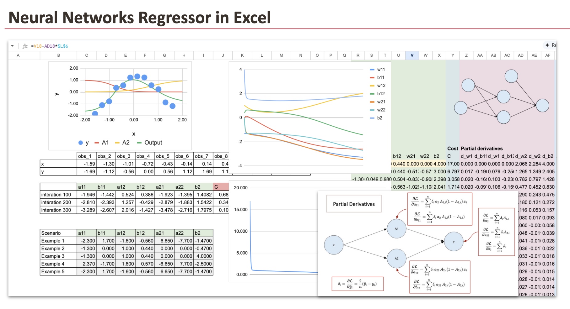
We will build a neural network regressor from scratch using Excel. Every computation will be explicit. Every intermediate value will be visible. Nothing will be hidden.
By the end of this article, you will understand how a neural network performs regression, how forward propagation works, and how the model can approximate non-linear functions using just a few parameters.
Before starting, if you have not already read my previous articles, you should first look at the implementation of linear regression and logistic regression.
You will see that a neural network is not a new object. It is a natural extension of these models.
As usual, we will follow these steps:
First, we will look at how the model of a Neural Network Regressor works. In the case of neural networks, this step is called forward propagation.
Then we will train this function using gradient descent. This process is called backpropagation.
1. Forward propagation
In this part, we will define our model, then implement it in Excel to see how the prediction works.
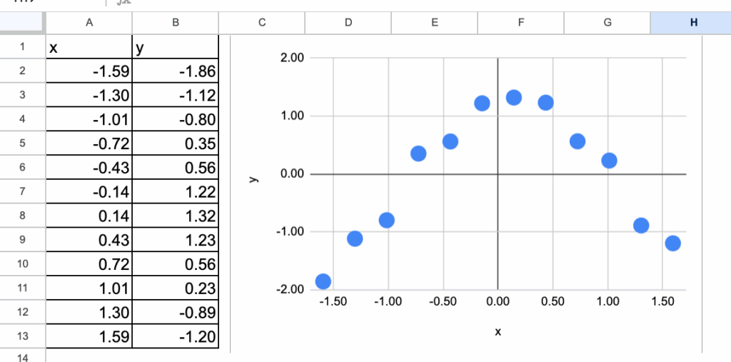
1.1 A Simple Dataset
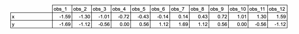
We will use a very simple dataset that I generated. It consists of just 12 observations and a single feature.
As you can see, the target variable has a nonlinear relationship with x.
And for this dataset, we will use two neurons in the hidden layer.
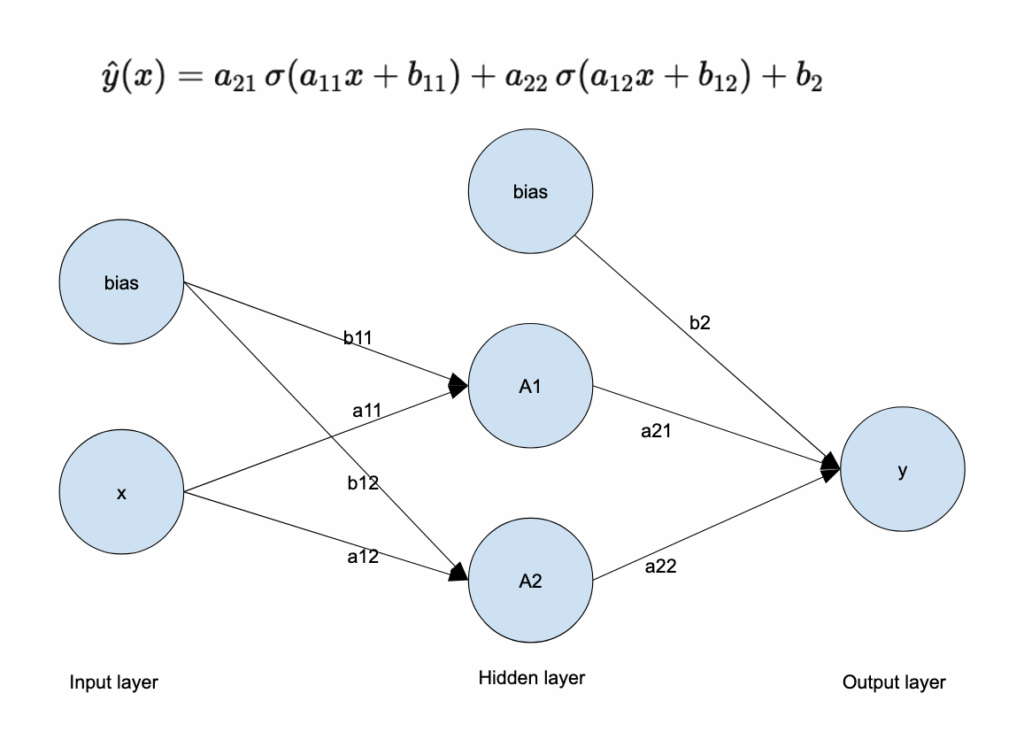
1.2 Neural Network Structure
Our example neural network has:
One input layer with the feature x as input
One hidden layer with two neurons in the hidden layer, and these two neurons will allow us to create a nonlinear relationship
The output layer is just a linear regression
Here is the diagram that represents this neural network, along with all the parameters that must be estimated. There are a total of 7 parameters.
Hidden layer:
a11: weight from x to hidden neuron 1
b11: bias of hidden neuron 1
a12: weight from x to hidden neuron 2
b12: bias of hidden neuron 2
Output layer:
a21: weight from hidden neuron 1 to output
a22: weight from hidden neuron 2 to output
b2: output bias
At its core, a neural network is just a function. A composed function.
If you write it explicitly, there is nothing mysterious about it.
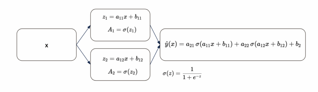
We usually represent this function with a diagram made of “neurons”.
In my opinion, the best way to interpret this diagram is as a visual representation of a composed mathematical function, not as a claim that it literally reproduces how biological neurons work.
Why does this function work?
Each sigmoid behaves like a smooth step.
With two sigmoids, the model can increase, decrease, bend, and flatten the output curve.
By combining them linearly, the network can approximate smooth non-linear curves.
This is why for this dataset, two neurons are already enough. But would you be able to find a dataset for which this structure is not suitable?
1.3 Implementation of the function in Excel
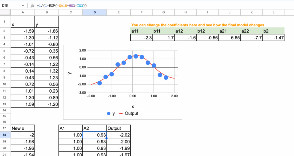
In this section, we will suppose that the 7 coefficients are already found. And we can then implement the formula we saw just before.
To visualize the neural network, we can use new continuous values of x ranging from -2 to 2 with a step of 0.02.
Here is the screenshot, and we can see that the final function fits the shape of the input data quite well.
2. Backpropagation (Gradient descent)
At this point, the model is fully defined.
Since it is a regression problem, we will use the MSE (mean squared error), just like for a linear regression.
Now, we have to find the 7 parameters that minimize the MSE.
2.1 Details of the backpropagation algorithm
The principle is simple. BUT, since there are many composed functions and many parameters, we have to be organized with the derivatives.
I will not derive all the 7 partial derivatives explicitly. I will just give the results.
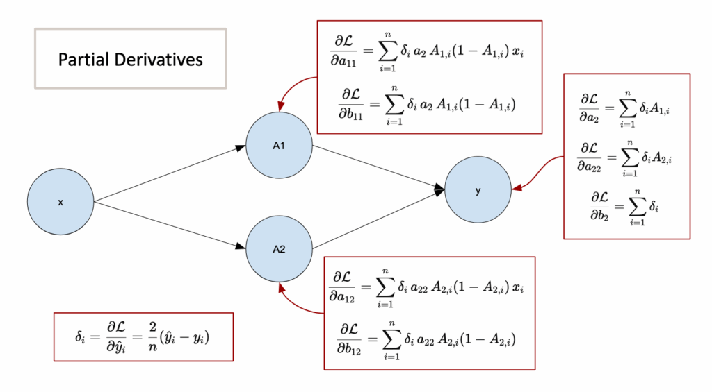
As we can see, there is the error term. So in order to implement the whole process, we have to follow this loop:
initialize the weights,
compute the output (forward propagation),
compute the error,
compute gradients using partial derivatives,
update the weights,
repeat until convergence.
2.2 Initialization
Let’s get started by putting the input dataset in a column format, which will make it easier to implement the formulas in Excel.
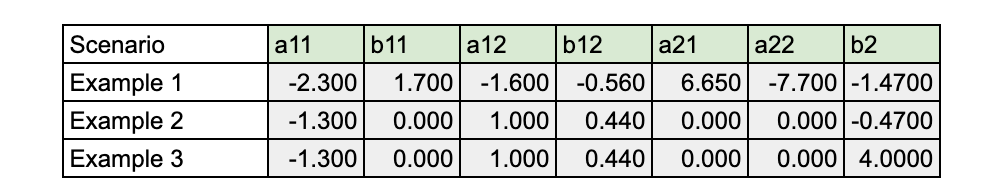
In theory, we can begin with random values for the initialization of the values of the parameters. But in practice, the number of iterations can be large to achieve full convergence. And since the cost function is not convex, we can get stuck in a local minimum.
So we have to choose “wisely” the initial values. I have prepared some for you. You can make small changes to see what happens.
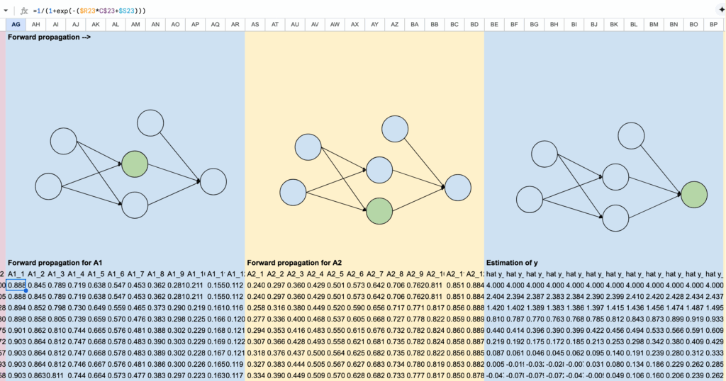
2.3 Forward propagation
In the columns from AG to BP, we perform the forward propagation phase. We compute A1 and A2 first, followed by the output. These are the same formulas used in the earlier part of the forward propagation.
To simplify the computations and make them more manageable, we perform the calculations for each observation separately. This means we have 12 columns for each hidden layer (A1 and A2) and the output layer. Instead of using a summation formula, we calculate the values for each observation individually.
To facilitate the for loop process during the gradient descent phase, we organize the training dataset in columns, and we can then extend the formula in Excel by row.
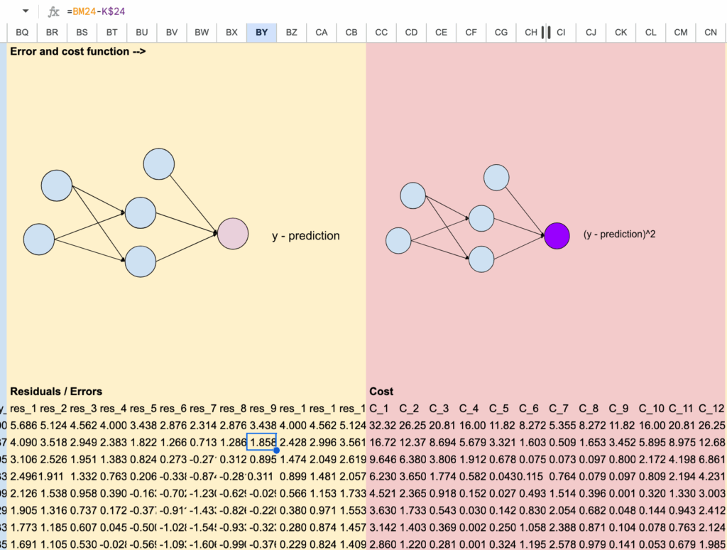
2.4 Errors and the Cost function
In columns BQ to CN, we can now compute the values of the cost function.
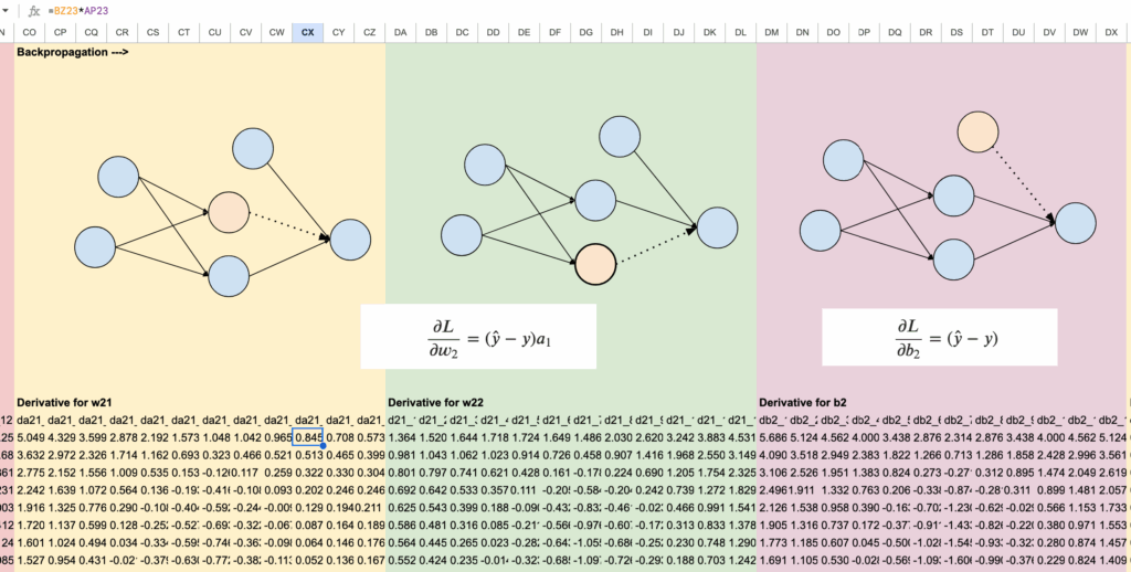
2.5 Partial derivatives
We will be computing 7 partial derivatives corresponding to the weights of our neural network. For each of these partial derivatives, we will need to compute the values for all 12 observations, resulting in a total of 84 columns. However, we have made efforts to simplify this process by organizing the sheet with color coding and formulas for ease of use.
So we will begin with the output layer, for the parameters: a21, a22 and b2. We can find them in the columns from CO to DX.
Then for the parameters a11 and a12, we can find them from columns DY to EV:
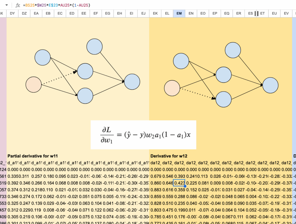
And finally, for the bias parameters b11 and b12, we use columns EW to FT.
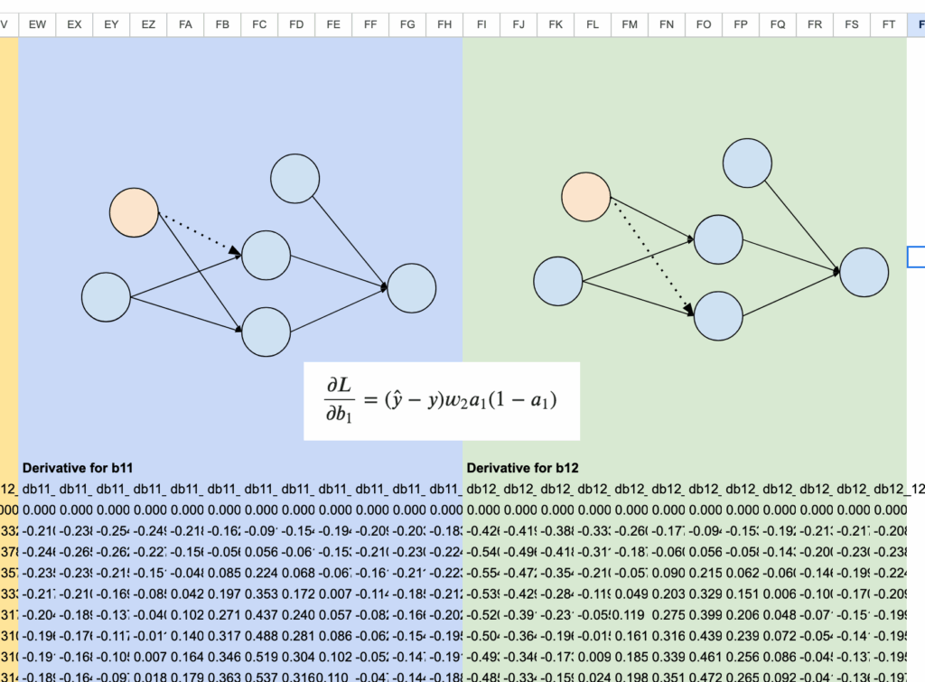
And to wrap it up, we sum all the partial derivatives across the 12 observations. These aggregated gradients are neatly arranged in columns Z to AF. The parameter updates are then performed in columns R to X, using these values.
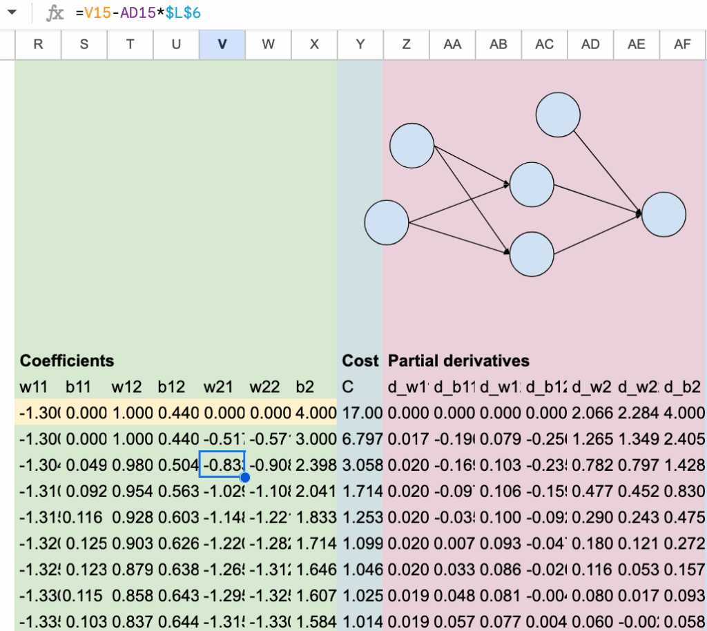
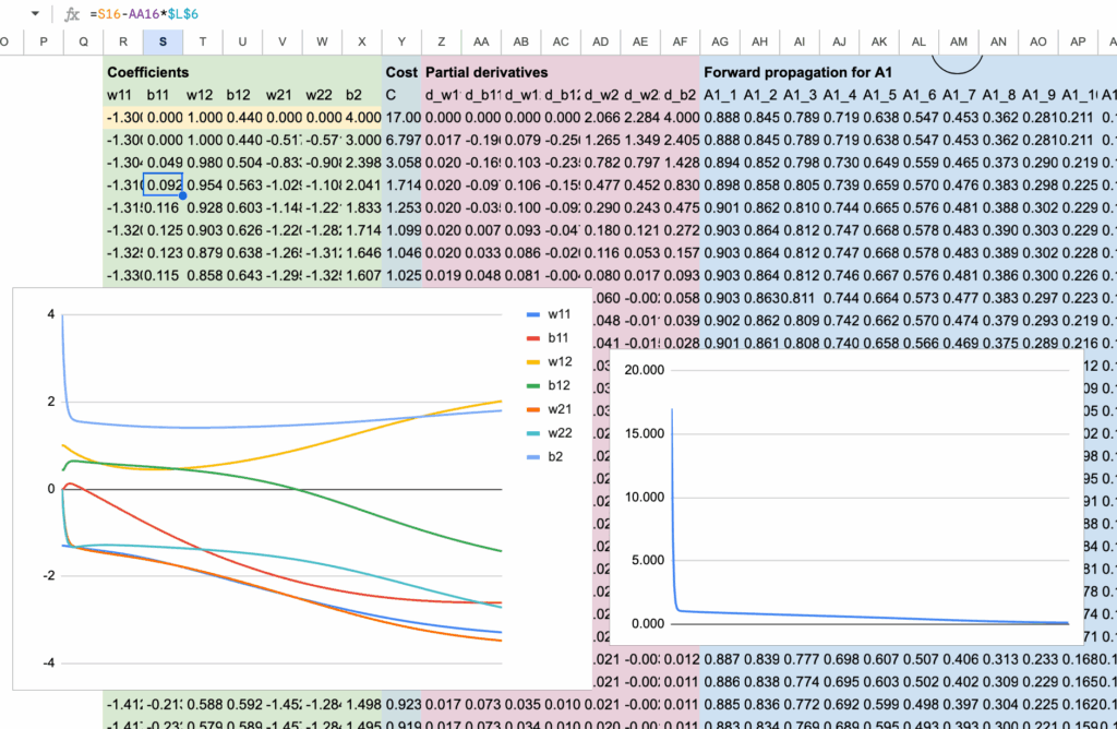
2.6 Visualization of the convergence
To better understand the training process, we visualize how the parameters evolve during gradient descent using a graph. At the same time, the decrease of the cost function is tracked in column Y, making the convergence of the model clearly visible.
Conclusion
A neural network regressor is not magic.
It is simply a composition of elementary functions, controlled by a certain number of parameters and trained by minimizing a well-defined mathematical objective.
By building the model explicitly in Excel, every step becomes visible. Forward propagation, error computation, partial derivatives, and parameter updates are no longer abstract concepts, but concrete calculations that you can inspect and modify.
The full implementation of our neural network, from forward propagation to backpropagation, is now complete. You are encouraged to experiment by changing the dataset, the initial parameter values, or the learning rate, and observe how the model behaves during training.
Through this hands-on exercise, we have seen how gradients drive learning, how parameters are updated iteratively, and how a neural network gradually shapes itself to fit the data. This is exactly what happens inside modern machine learning libraries, only hidden behind a few lines of code.
Further Reading
Already Day 17 of my Machine Learning “Advent Calendar“.
People usually talk a lot about supervised learning, unsupervised learning is sometimes overlooked, even though it can be very useful in many situations. These articles specifically explore these approaches.
An improved and more flexible version of k-means.
Unlike k-means, GMM allows clusters to stretch, rotate, and adapt to the true shape of the data.
But when do k-means and GMM actually produce different results?
Take a look at this article to see concrete examples and visual comparisons.
Local Outlier Factor (LOF)
A clever method that compares each point’s local density to its neighbors to detect anomalies.
All the Excel files are available through this Kofi link. Your support means a lot to me. The price will increase during the month, so early supporters get the best value.
 All Excel/Google sheet files for ML and DL