
Here we provide details of the experimental setup and the algorithmic choices made in this study. We begin by describing the device used for our experiments. We then follow with a discussion of the intelligent computational approaches used in the algorithm. Finally, details of each stage are discussed. An overview of all the stages of the algorithm is given in Extended Data Table 1.
Hyperparameters that are not explicitly given here are provided in Supplementary Section 5.
Device and measurement details
The device consists of a Ge–Si core–shell nanowire lying on top of nine bottom gates measured in a variable-temperature insert in a liquid-helium bath, with the sample mounted below the 1-K pot (base temperature, 1.5 K). By applying positive voltages to the first five bottom gates from the left, an intrinsic hole gas inside the nanowire is depleted to form a hole DQD. A scanning electron microscopy image of a device similar to the one used here is shown in Extended Data Fig. 1. The device, measurement apparatus and pulse sequence are the same as those used in ref. 41 and are described in detail in that work, which was performed independently and served primarily as an initial reference for the device’s characteristics. We did not explicitly encode knowledge of the particular qubit from ref. 41 into our algorithm.
To amplify the measurements that rely on an MW pulse, we applied pulse modulation by a lock-in amplifier at 87.777 Hz. The measurements, therefore, have an in-phase and out-of-phase component. We apply principal component analysis to these measurements and project each measurement onto the principal axis. We further offset the measurements such that they are strictly positive. Measurements that are obtained in this way are marked as ILI, as opposed to currents that were measured conventionally (which are marked as ∣I∣).
Techniques used in the algorithm
Useful automation of tuning from a de-energized device to identify Rabi oscillations requires an algorithm that can adapt to different data-capture regimes, and be transferred to other, similar devices. To achieve this, we have made extensive use of intelligent, adaptive and data-driven subroutines. Nowadays, there is a plethora of such techniques to choose from. To choose the right technique to apply to each stage of the algorithm, we considered the following:
the need for expert-labelled training data, which was not always possible or realistic to source;
the need of being efficient in both total number of measurements taken during a stage and in the resources needed for computing decisions about which measurements to take;
the minimal accuracy needed in each stage for the whole algorithm to be able to achieve its overall goal of identifying operating parameters for a qubit.
To address the above considerations across the many stages of the algorithm, a non-exhaustive list of techniques we have found useful to use includes GP inference, convolutional neural networks (CNNs), unsupervised computer vision and computational geometry techniques, and Bayesian optimization. We now briefly introduce these, highlighting their strengths and weaknesses.
GPs are a popular form of non-parametric Bayesian inference54. They can be thought of as a method for doing principled Bayesian inference over a space of functions. GPs can be tailored to any specific domain or problem by making a choice of the so-called kernel (or covariance) function, a part of this model that describes prior knowledge about the possible space of functions in which inference is to occur. This choice can allow practitioners to encode important domain knowledge before capturing any data, such as specifying knowledge of periodicities, symmetries or the expected degree of smoothness of the underlying process that is being observed. This constitutes the main strength of GP modelling, often enabling highly data-efficient inference. However, both model fitting and model prediction can be computationally intensive, typically growing cubically54 in the number of observed data points.
Over the past two decades, CNN architectures have proved to be go-to models for solving computer vision tasks. Their strengths lie in their adaptability across different computer vision tasks, their robustness in the face of unknown noise and their computational efficiency at training time. Their weakness lies in always requiring substantial amounts of training data. In this work, we use some standard architectures, such as ResNet55, as tools for extracting properties from or making assessments of stability diagrams. Where we have applied them, training data have been either generated by a sufficiently good simulator or gathered from this or similar devices and then labelled by an expert.
Often, the use of CNNs is neither required nor appropriate for the particular computer vision task at hand. In particular, it has been of crucial importance to a number of stages through the algorithm to be able to automatically locate and segment bias triangles within stability diagrams using a coordinate-wise approach. To achieve this, we have used a number of unsupervised computer vision techniques that can mitigate noise in, and localize features of the geometric figures present in the stability diagrams. Although CNNs would require large amounts of labelled training data to achieve this result, the requirements can be met by computer vision techniques that need no training data, and require only a few hyperparameter choices to be made. All together, we have called this a bias triangle segmentation framework, and it is described in ref. 49, where the specific application to PSB detection is also detailed.
Bayesian optimization21,22,56,57 is a general, iterative approach to black-box function optimization. At each iteration, it constructs a surrogate model of the function being approximated using the data already gathered, and uses this surrogate model to efficiently compute the next most informative location from which to sample the unknown function. To apply this technique, one must specify a score function to optimize and a parameter space over which the search for an optimum is conducted. The choice of the surrogate model is also influential in the accuracy, efficiency and reliability achieved using this method. In this work, we have made consistent use of GP surrogate models using a Matern 5/2 kernel.
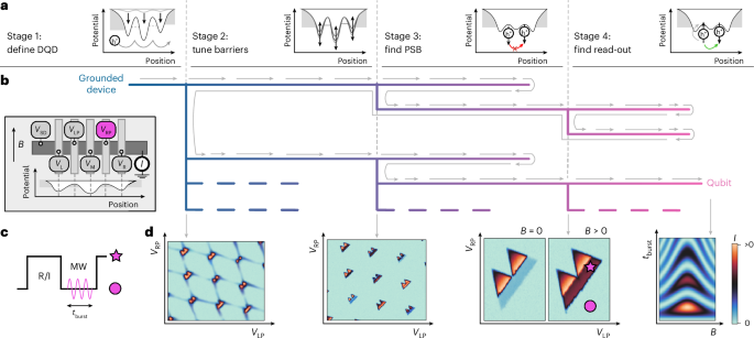
Stages of the algorithmStage 1: define DQD
(a) Hypersurface building. As the first step, the algorithm determines a current that it considers to be pinched off by ramping to the high end of the safe ranges. We take repeated current measurements there to characterize the noise floor. From the noise floor, we compute a pinch-off current.
Next, we sample several points within the safe ranges using a Sobol sequence for quasi-random locations. The points are used to define rays from the origin that are then investigated for pinch-off. To avoid overloading the current amplifier, we search for pinch-off from the origin towards the upper end of the safety ranges with a low bias voltage. Once the pinch-off is found, we retrace with a higher bias voltage to confirm the exact pinch-off location.
Finally, we use these data to construct the hypersurface model, as outlined in the main text.
(b) Double-dot detection. The previous stage defines a region within which we can look for a DQD potential. We sample quasi-random points via a Sobol sequence for investigation. For each point, we vary both plunger voltages simultaneously and measure the current, following the method described in ref. 21. We use the random forest classifier developed in ref. 22 to check for the presence of Coulomb peaks. If Coulomb peaks are found, we then measure a stability diagram. This diagram is analysed with a neural network to detect features of the DQD. The neural network was trained on data from a variety of devices, mainly from the data gathered in refs. 21,22, and additional data are obtained from a nanowire device different from the one used in this work. In total, there were 4,611 stability diagrams, out of which 726 showed double-dot features.
Stage 2: tune barriers
(a) Barrier optimization. On the formation of separated pairs of bias triangles, we perform coordinate-wise segmentation and polygon fitting49 to facilitate their tracking and feature extraction throughout the remainder of the tuning pipeline.
Segmentation and shape extraction enable the assessment of the current intensity difference between the baseline and gap formed between the base and first excited-state line. By quantifying this intensity difference in a base separation score, we can use a Bayesian optimization framework, which seeks to maximize the intensity difference, as a promising indicator for detecting viable candidates for PSB.
Each pair of bias triangles should present a base well separated from the main body. By measuring the d.c. current through the device, we effectively probe the internal energy transitions between the two quantum dots. Crucially, these transitions remain relatively unaffected by the thermal broadening of the leads, making the scheme viable at higher (‘hot’) temperatures. For PSB-based read-out to be effective, the energy splitting between the relevant singlet and triplet states, that is, ΔST, must exceed the thermal energy (kBT). Once ΔST ≤ kBT, the PSB mechanism can degrade and allow unwanted leakage current, thereby compromising the quality of the read-out. The energy-splitting score, therefore, serves as a metric to guide the algorithm towards bias triangles that are more likely to yield robust spin read-out and, ultimately, stable qubit operation. Supplementary Section 3 provides further discussion on the relation of this score with spin-state visibility. Supplementary Section 4 provides empirical justification of the score.
The separation score is computed by averaging the current along the detuning axis (Fig. 2b(ii) shows two one-dimensional traces), and computing the ratio of the intensity between the peaks and the lowest point in the valley between them. In the case of multiple triangles, the highest separation is used as the score.
Certain potential landscapes can lead to situations in which charge configurations are affected by charge switch noise. Since these potentials are unlikely to be used as a qubit and the resulting bias triangles can skew our base separation scoring, we excluded them by leveraging a neural network classifier. This classifier was trained to distinguish between normal bias triangles and the ones that are affected by charge switch noise (Extended Data Fig. 2). The training dataset for this classifier was obtained as follows: initially, potential bias triangles were identified using our segmentation routine. Subsequently, we manually labelled 2,302 of these (1,539 samples showed no switch noise) to create a robust training set. The classifier itself was then obtained by fine-tuning a ResNet-based architecture with this dataset.
Once the voltage space has been explored through Bayesian optimization, we have a clear understanding of the landscape (Fig. 2b(ii)). The measurements in this optimization were obtained using an efficient measurement algorithm (Supplementary Section 6). We sample the most promising regions again without the efficient measurement algorithm and analyse them, as described in the next section.
(b) Plunger window selection. Given a sampled stability diagram containing bias triangles, the aim is to select the region that contains as many bias triangles with scores as high as possible, no areas with current that is too high and as few switches as possible (Fig. 2b(iii)). High-current bias triangles are unlikely to be able to be used for qubit operations. This is a heuristic and we set a conservative threshold of 200 pA. To ease the downstream steps, the region should be a rectangular window. Through an iterative approach, starting from the smallest bounding boxes containing each single pair of bias triangles, larger windows are constructed by merging the existing ones in case they satisfy the conditions about switch absence and low currents. For the absence of switches, we used a soft constraint, allowing for bias triangles affected by switch noise in case their total area was less than 25% of the area covered by all triangles in the window. The algorithm complexity scales exponentially with respect to the number of triangles and some heuristics have been leveraged to reduce substantially complexity and, therefore, execution time. In particular, at each iteration, only the top 100 bounding boxes by the number of contained triangles without switches were kept, to ensure a manageable upper limit on the number of possible merges. The routine halts when no further merges are possible. Once the plunger windows have been selected, they are ranked by the highest separation score.
Stage 3: find PSB
(a) Wide-shot PSB detection. To identify each bias triangle’s location, we first leverage the fact that they sit on a honeycomb or skewed rectangle pattern. We use autocorrelation on the stability diagram to identify this pattern. The largest two peaks in the autocorrelation help us establish a vector that spans this pattern of skewed rectangles. To fix the pattern in place, we use a blob detection algorithm, using the first blob it identifies. This helps us accurately overlay the skewed rectangle pattern and estimate the locations of the bias triangles (Extended Data Fig. 3).
Next, we extract these bias triangles using the identified locations, with side lengths informed by the pattern dimensions. These extracted bias triangles are then input into a neural network for further analysis. We used autonomously gathered data that were taken during the initial development phase. In total, we used 626 pairs of bias triangles taken from 70 stability diagrams. Here 55 pairs of bias triangles showed PSB. Reference 38 provides more detailed information on this procedure.
(b) Re-centring and high-resolution PSB detection. In an effort to filter the previously detected candidates for PSB and eliminate false positives, a second set of higher-resolution measurements is performed. For that purpose, a dedicated low-resolution stability diagram of the candidate bias triangles is taken and used to update the plunger voltage extent based on the detected contours, effectively performing a re-centring. With the updated voltage extent, high-resolution stability diagrams with B = 0 T and with B = 0.1 T are taken.
A second substage of PSB classification is applied through a segmentation-based detection and feature extraction framework, which facilitates the coordinate-wise quantification of geometric and physical properties of bias triangles49. In particular, given the high-resolution stability diagram with B = 0.1 T, this framework fits minimum-edge polygons to the detected contours of bias triangle pairs by utilizing a relaxed extension of the Ramer–Douglas–Peucker algorithm49. Once the segmented shape mask is identified, further geometric properties such as the base and excited-state lines can be automatically extracted solely based on prior knowledge of the bias voltage sign, which predicts the direction in which the bias triangles point.
For the identification of PSB, an analytical classifier based on the above framework was devised49. PSB expresses itself as a suppressed baseline of the bias triangles at B = 0 T. At B > 0 T, there is a leakage current at the baseline. The routine extracts the segment enclosing the base and a prominent excited-state line on the stability diagram with a leakage current (B = 0.1 T). Subsequently, the average pixel intensity of the segment normalized by the intensity of the entire pair of bias triangles is computed. By superimposing the detected segment on the scan with blocked current (B = 0 T), normalized intensity values are compared and, if their difference exceeds a specified threshold, the charge transition is identified as positive for PSB.
On the basis of the segmented shape mask of the bias triangle, further geometrical properties can be automatically extracted, which enables the tuning of bias triangle features in stage 2. The detuning axis, utilized for the Danon gap measurement, is automatically extracted by identifying the bias triangles’ base midpoints and tips and computing the lines between them.
(c) Danon gap check. As a further filter for possible candidates, we check to find the magnetic field dependence of the leakage current at the base of the bias triangles in a different way. As a function of the applied magnetic field B, we expect the leakage current to be minimal at B = 0 T and higher away from this point. We call this the Danon gap58. A current measurement of the detuning line as the magnetic field is varied, giving us a two-dimensional input (Extended Data Fig. 4), which we can analyse as follows. Ignoring the noise signal, the current is roughly constant along the magnetic field axis, whereas the detuning line axis is information rich. Away from the Danon gap, there are two local extrema (to one side, the noise floor outside the bias triangles, and to the other side, the gap due to singlet–triplet energy splitting), whereas the Danon gap region is characterized by a monotonic behaviour, with roughly a constant value.
To detect the presence of the Danon gap, the current I is first processed with a Gaussian filter, to smooth out the noise, and then the absolute slopes along the detuning line axis are integrated: \(g(B):={\sum }_{\varepsilon }\left|\frac{\partial \widetilde{I}(\varepsilon ,B)}{\partial \varepsilon }\right|\), where the derivative is the discrete derivative along the detuning line axis. The function g is minimized in the areas where the smoothed signal \(\widetilde{I}\) shows a constant value. We show the normalized function \({\bar{g}} =\frac{g}{| \varepsilon | }\) in Extended Data Fig. 4. To detect the presence of the Danon gap from g, two tunable hyperparameters are used, validating the depth and width of the basin of the global minimum of g: in case the basin is not prominent enough, there is no Danon gap. As the last check, the location of the minima has to be in proximity of zero magnetic field.
Stage 4: find read-out
(a) Tracking and entropy optimization. In the subsequent steps, we apply a pulse sequence to the right plunger electrode. As it is a two-stage pulse, the bias triangles will have a ‘shadow’ in the stability diagram. We need to identify the original bias triangles and find a suitable region in which we can expect to find qubit read-out. In light of the resulting shape distortions and further degrading effects to the measurement quality, we opt for template matching as opposed to performing re-segmentation for bias triangle tracking to ensure robustness.
The relative direction in which the shadow bias triangles appear with respect to the original one is known in advance due to the applied pulse shape. This is incorporated into the shape-matching approach as the cardinal direction to uniquely identify and track the triangles. We perform shape matching by comparing the edge map of a stability diagram before pulsing, functioning as the template, to the edge map of a subsequent stability diagram with pulsing, functioning as the source for current information. Further, we extract the segmented shape mask from the template. The method slides the template over the source edge map, thereby comparing the template with individual patches of the stability diagram with pulsing, and returns a result matrix (of the same size as the source) whose individual entries quantify the similarity with the template patch. The used similarity metric is the normalized correlation coefficient, and the patch with the maximum correlation is selected. Once the appropriate patch has been identified, the initial segmentation mask of the stability diagram without pulsing is mapped to the stability diagram with pulsing and used for subsequent processing.
To identify the optimal read-out spot, we extract the segment enclosing the base and prominent excited-state lines on the obtained segmented mask of bias triangles with pulsing. We then perform Bayesian optimization of a read-out quality score over the following parameters: the constrained two-dimensional plunger gate voltage space, frequency of the driving pulse fMW and burst time tburst.
Optimal read-out candidates are those that meet the resonance conditions of the qubit. If they are met, there is a leakage current that we record using the lock-in amplifier. For a given burst time tburst (relating to the Rabi frequency fRabi) and a given frequency of the driving pulse fMW (relating to the g-factor), the leakage is characterized as a peak in leakage current for a certain magnetic field B. In this setup, hardware-related resonances and non-uniform attenuation across certain frequency ranges introduce distortions when the drive frequency is varied instead of the magnetic field. Consequently, sweeping the magnetic field at a fixed frequency provides a more stable and interpretable signal, even though it is slower. Thus, for read-out optimization, we measure the current with varying magnetic fields. Instead of applying principal component analysis, as explained above, we use the L2 norm of the in-phase and out-of-phase components to retrieve a one-dimensional trace l(B). This guarantees peaks to be higher than the background, as opposed to processing with principal component analysis, which can lead to dips rather than peaks.
To quantify the sharpness of these peaks, we developed a score based on the Shannon entropy \(H=-{\sum }_{B}\left[l(B)\log [l(B)]\right]\) of the trace. For the calculation of the entropy of the score, we first subtract the median and then clip values at zero. This particular preprocessing turns the trace into something more akin to a distribution and enhances the robustness of our score, making it less susceptible to potential noise disturbances in the trace. This method results in a smooth score landscape suitable for Bayesian optimization.
(b) Resonance confirmation. This verification step acts as a final filter and all the last stages are executed once a candidate passes this filter. The previous stage sends a candidate with a suspected resonance condition. The stage re-measures the leakage current as a function of the magnetic field. If the resonance condition was truly found, a peak should appear at the same magnetic field again. If we detect a peak with a specified prominence at this magnetic field within a set margin of error, the resonance condition is considered confirmed and all downstream measurements are executed. We note that a noisy candidate might pass this stage. Repeating the verification step can reduce such occurrences.
(c) Qubit measurements. Once a resonance condition is found, we vary the magnetic field and burst duration. The characteristic Rabi chevron can be analysed by considering the frequency spectrum for each magnetic field. The frequency should have a minimum at the magnetic field that meets the resonance condition of the qubit. The amplitude should also be the maximum there due to decoherence for off-resonant driving. We can, therefore, simply look for the maximum amplitude in the Fourier-transformed Rabi chevron (Extended Data Fig. 5). This information will give us the precise resonance conditions for the last step, which are repeated measurements of Rabi oscillations on resonance.
Characterization
The maps shown in Fig. 3 were generated using automated measurements. Initially, on identifying a qubit, we record its read-out spot, g-factor and fRabi. We then alter the confinement potential by slightly adjusting the barrier gate voltages. This adjustment may shift the bias triangles, consequently moving the read-out spot, g-factor and fRabi. Our method involves tracing these transitions to locate the read-out spot in its new position. At this new location, we conduct an electric dipole spin resonance check scan. Any changes in the peak’s location inform us about variations in the g-factor. Furthermore, measuring Rabi oscillations at this point helps update our understanding of fRabi.
As we progressively deviate from the initial measurement point, we utilize our closest prior qubit data to infer the properties at the new location. This step is crucial as a shift in the g-factor necessitates modifying the magnetic field range, whereas a change in fRabi requires adjusting the tburst duration for the electric dipole spin resonance check to accurately detect resonances.