
To create a multimode optomechanical system, a silica bead of nominal diameter 100 nm is levitated in high vacuum using a 150 mW Gaussian beam (wavelength 1064 nm) tightly focused by a high NA (0.77) aspheric lens. The experiments are conducted at the pressure of 1 × 10⁻⁵ mbar to mitigate mechanical interactions with the surrounding gas molecules. The simplified experimental scheme is illustrated in Fig. 1a, with a collimated input trapping beam incident on a high NA lens, the converging beam forms a three dimensional trapping potential about the focal point of the objective. A more detailed schematic of the experimental setup can be found in the supplementary material [Supplementary Note I]. For a bead size much smaller than the trapping beam wavelength, the nanoparticle can be approximated as an electric dipole and is subjected to the gradient force leading to dynamics about the electric field intensity maximum36. The trapping potential well created by the gradient force is asymmetric in the transverse plane if the input beam is linearly polarized, and the potential well tends to elongate in the direction of polarization37, see the left panel of Fig. 1b. The different trapping potentials in the x and y directions result in distinct oscillation frequencies in the x and y directions, which are Ωx/2π = 115 kHz, and Ωy/2π = 130 kHz, respectively, in our experiment.
Fig. 1: Demonstration of the experimental methods.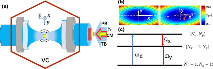
a Illustration of a nanoparticle optically levitated by a trapping laser beam (TB) inside a vacuum chamber (VC), with a probe beam (PB) measuring its position. The x and y transverse oscillation modes can be coupled by coherent modulation (CM) of the trapping laser. The nonlinear parametric cooling (γc) is selectively exerted on the nanoparticle in the x and y-directions and the corresponding rates are expressed by γcx and γcy respectively, which can be different or identical. The z-motion is frozen out by feedback cooling and is not considered in our model. b Left panel: The asymmetric trapping potential well in the x − y plane that results from a linearly polarized trapping beam. Right panel: Coupling of the two transverse modes created by periodically rotating the potential by a small angle θ. c The energy level diagram showing phonon down-conversion process ωd = Ωx + Ωy, where ωd is the driving frequency, Ωx,y(Nx,y) are the oscillation frequencies (phonon numbers) of the x and y modes, respectively.
The coupling between the x and y modes is introduced by periodically rotating the trapping potential well in the transverse plane about the z-axis by a small angle \(\theta=\delta \cos \left({\omega }_{d}t+{\phi }_{d}\right)\), as illustrated in the right panel of Fig. 1b, where the polarization rotation is modulated harmonically with small amplitude δ, driving frequency ωd, and phase ϕd. The Hamiltonian of this coupled mode system can be presented as (all theoretical equations are detailed in the Supplementary Information):
$${H}_{tot}= \hslash {\Omega }_{x}{\widehat{b}}_{x}^{{{\dagger}} }{\widehat{b}}_{x}+\hslash {\Omega }_{y}{\widehat{b}}_{y}^{{{\dagger}} }{\widehat{b}}_{y}\\ -\hslash {\Omega }_{xy}\cos ({\omega }_{d}t+{\phi }_{d})({\widehat{b}}_{x}^{{{\dagger}} }+{\widehat{b}}_{x})({\widehat{b}}_{y}^{{{\dagger}} }+{\widehat{b}}_{y}),$$
(1)
where \({\widehat{b}}_{i}^{{{\dagger}} }\) and \({\widehat{b}}_{i}\) are the corresponding bosonic annihilation and creation operators of the two modes (i = x or y), \({\Omega }_{xy}=\left({\Omega }_{y}^{2}-{\Omega }_{x}^{2}\right)\delta /(2\sqrt{{\Omega }_{x}{\Omega }_{y}})\) is the coupling strength proportional to the rotating angle δ. Parametric driving is accomplished by setting the driving frequency approximately equal to the summation of the two modes oscillation frequencies: ωd = Ωx + Ωy. To maximize the squeezing rate, the driving phase will later be set to ϕd = 0. In the interaction picture and using the rotating wave approximation, Eq. (1) simplifies to:
$${H}_{tot}=-\frac{\hslash {\Omega }_{xy}}{2}({e}^{-i{\phi }_{d}}{\widehat{b}}_{x}^{{{\dagger}} }{\widehat{b}}_{y}^{{{\dagger}} }+{e}^{i{\phi }_{d}}{\widehat{b}}_{x}{\widehat{b}}_{y}).$$
(2)
Equation (2) describes the nondegenerate parametric oscillation that generates down-converted phonons in the transverse modes. The process is illustrated by the energy level diagram shown in Fig. 1c. Sum-frequency coupling drives the system into an upper energy level and coherent phonons with frequencies Ωx and Ωy are produced during the down-conversion process.
The parametric amplifier commonly displays instability beyond a pump threshold, characterized by a divergent increase of oscillation amplitude15,38. This phenomenon extends to our levitated nanoparticle. Driven solely by mode-coupling, the motion of the particle in the transverse plane undergoes unstable amplification, resulting in rapid loss from the trap. To counter this, we apply nonlinear parametric cooling to balance the parametric driving and stabilize the nanoparticle oscillation.
The dynamics of this two-mode system can be expressed by the master equation for the density matrix ρ
$${\rho }^{\cdot }=-\frac{{{{\rm{i}}}}}{\hslash }[{H}_{tot},\rho ]+{{{\mathcal{L}}}}\rho,$$
(3)
where the detailed form of the Lindblad term \({{{\mathcal{L}}}}\rho\) can be found in the Supplementary Note II. For further analysis, we transform the master equation of Eq. (3) to the quantum Langevin equations via quantum state diffusion theory39,40, which yields,
$$\frac{{{{\rm{d}}}}}{{{{\rm{d}}}}t}{Q}_{x(y)}= {\Omega }_{x(y)}{P}_{x(y)}\\ \frac{{{{\rm{d}}}}}{{{{\rm{d}}}}t}{P}_{x(y)}+ 2\left({\gamma }_{g}+3{\gamma }_{cx(y)}{Q}_{x(y)}^{2}\right){P}_{x(y)}+{\Omega }_{x(y)}{Q}_{x(y)}-2{\Omega }_{xy}\cos ({\omega }_{d}t+{\phi }_{d}){Q}_{y(x)}\\ = {\xi }_{x(y)}(t),$$
(4)
where \({Q}_{k}={\widehat{b}}_{k}^{{{\dagger}} }+{\widehat{b}}_{k}\) and \({P}_{k}={{{\rm{i}}}}\left({\widehat{b}}_{k}^{{{\dagger}} }-{\widehat{b}}_{k}\right)\), \(\left(k=x,y\right)\) are the generalized positions and momenta of the x and y modes, γg is the gas damping rate, γci are the nonlinear parametric cooling rates for the mechanical modes, where i = x or y, ξi(t) is the noise caused by the thermal environment, the trapping laser, and the feedback cooling. All theoretical results in this paper were found by analytically or numerically solving Eqs. (4).
First, we characterize the system both in the absence as well as in the presence of mode coupling. The temporal evolution of the mean phonon number in the two modes is presented in Fig. 2a. The mean phonon number is measured by \(\langle {N}_{i}\rangle=M{\Omega }_{i}\langle {q}_{i}^{2}\rangle /\hslash\), where M is the mass of the levitated particle, qi is the displacement of the particle’s center of mass with respect to the center of the trap, ℏ is the reduced Planck’s constant, and i = x or y. The feedback cooling is active throughout the 200 ms experiment, allowing ample time for the system to first relax to a low energy state, shown as the gray region between 0 ~ 30 ms. We initiate the parametric drive at 30 ms and subsequently terminate the parametric drive at 200 ms. This cycle is iterated 100 times, and the average plus minus one standard deviation of these 200 ms traces is depicted as shaded blue and red areas in Fig. 2a. In the trace, the mean phonon number is decreasing in the first 30 ms due to the gas damping and feedback cooling. Once the parametric drive (mode-coupling) is applied at ~ 30 ms, the mean phonon numbers in the x and y modes begin to increase and finally stabilize at nearly identical levels, resulting from the balance between the parametric drive and nonlinear parametric cooling. The red and blue solid lines shown in Fig. 2a are the theoretical predictions found by solving Eq. (4) numerically with the phonon numbers defined as \({N}_{i}=({P}_{i}^{2}+{Q}_{i}^{2})/4\), i = (x, y). These predictions fit quite well with the experimental data (the details of the theoretical predictions can be found in the Supplementary).
Fig. 2: Two-mode phonon laser characterization.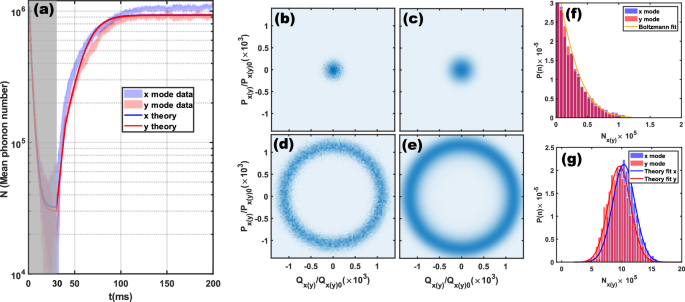
a Evolution of the mean phonon number as a function of time. The nonlinear parametric cooling is on throughout. The parametric drive is switched on at 30 ms. The solid curves are theoretical predictions and the red and blue shaded areas represent the standard deviation around the average of the experimental data. The process was repeated 100 times and averaged to generate this data. b, d are the scattering plots of in-phase and quadrature component of particle’s motion obtained from the experiment, (b) is recorded before the mode-coupling while (d) is after the mode-coupling is turned on. c, e are the theoretical steady state phase space distributions before and after the coupling is turned on. A phase transition from Brownian motion to coherent oscillation is evident in both experiment and theoretical plots. Note that while (b–e) represent x mode data, the y mode has a very similar distribution. f The phonon number distribution of the x and y modes in the absence of coupling, where both modes are in the thermal state and fitted by a Boltzmann distribution. g The phonon number distribution of the x and y modes in the presence of coupling, where both modes are coherent and are fitted by nearly Poissonian distributions.
The phase-space distributions were obtained by measuring the in-phase Q and quadrature P components of the oscillation signal of the nanoparticle, scaled by the zero point position (Q0) and momentum (P0) spread of the oscillator modes, as shown in Fig. 2b, d. In the absence of coupling (Ωxy = 0), the distributions for both x and y are disks with their center at the origin, corresponding to the thermal distributions. In the presence of coupling, the phase space distributions take the shape of annuli with much larger radii than the thermal states, and correspond to phase-diffused coherent states. It is evident that the phonons generated without mode-coupling are thermal, while those generated with mode-coupling are coherent, and that there is a phase transition between the two regimes, see Fig. 2b, d. We emphasize that the experimental data in Fig. 2b, d can represent either the x or the y mode. The two show very similar behavior without and with coupling and overlap each other in the phase space distribution plot. The theoretical marginal phase-space distributions associated with the experimental data in Fig. 2b, d are predicted based on the oscillators’ P-function distributions41:
$$\phi ({N}_{x})={{{\mathcal{N}}}}\frac{\pi {A}_{t}}{2{\gamma }_{gy}}{{{\rm{Exp}}}}\left\{-\frac{2}{{A}_{t}}\left[3{\gamma }_{cx}{N}_{x}^{2}-\left(\frac{{\Omega }_{xy}^{2}}{4{\gamma }_{gy}}-{\gamma }_{gx}\right){N}_{x}\right]\right\},$$
(5)
$$\phi ({N}_{y})={{{\mathcal{N}}}}\frac{\pi {A}_{t}}{2{\gamma }_{gx}}{{{\rm{Exp}}}}\left\{-\frac{2}{{A}_{t}}\left[3{\gamma }_{cy}{N}_{y}^{2}-\left(\frac{{\Omega }_{xy}^{2}}{4{\gamma }_{gx}}-{\gamma }_{gy}\right){N}_{y}\right]\right\},$$
(6)
where \({{{\mathcal{N}}}}\) is the normalization constant, At is the rate of photon scattering from the trapping beam, and γgi(γci) are the gas damping (nonlinear parametric cooling) rates for the x and y modes, respectively, with i = (x, y). More details about the P-function can be found in the supplementary material [Supplementary Note III]. As can be seen in Fig. 2(c), (e), the theoretical predictions agree with the experimental data.
The experimental phonon number probability distributions are shown in Fig. 2f, g. As can be seen, in the absence of coupling, the distribution is Boltzmannian, indicating both modes to be in the thermal state. In the presence of coupling, the phonon number distribution exhibits super-Poissonian statistics as the mean and variance of the phonon number distribution are Nm = 1.06 × 10⁶ and \({\sigma }_{n}^{2}=(1.5\pm 0.2)\times 1{0}^{10}\), respectively. The variance of the corresponding thermal state is given by \({N}_{m}^{2}+{N}_{m}\approx 1{0}^{12}\). Since our experimental data shows a smaller variance than this, we observe subthermal phonon number squeezing in each mode. Theoretical predictions can readily be obtained for the phonon number probability distributions by using Eqs. (5) and (6), and as can be seen from Figs. 2(f) and (g) they agree quite well with experiment.
Importantly, the location of the transition from thermal to coherent behavior can be found by setting \({\Omega }_{xy}^{2}/(4{\gamma }_{gy(x)})-{\gamma }_{gx(y)}=0\) (at which value the phase space disk turns into an annulus) in Eqs. (5) and (6), which yields the threshold modulation \({\delta }_{th}=4\sqrt{{\gamma }_{gx}{\gamma }_{gy}{\Omega }_{x}{\Omega }_{y}}/({\Omega }_{y}^{2}-{\Omega }_{x}^{2})\). We now consider the important role played by this threshold value. First we note that, although not displayed here, the phase space distributions for non-zero coupling values below the threshold were also observed to be thermal, i.e., the same as in the absence of coupling. The states with coherence were only obtained above threshold, as in Figs. 2b–e. To further clarify the role of the threshold, the mean steady state phonon number in each mode was next determined as a function of the normalized parametric driving modulation rc = δ/δth. The corresponding experimental data is shown in Fig. 3(a), indicating an initially flat region, followed by a threshold near δ = δth and finally a linear increase. The theoretical values of the mean phonon numbers were obtained from ϕ(Nx) and ϕ(Ny) in Eqs. (5) and (6), considering the generalized amplitude \({r}_{i}=\sqrt{{N}_{i}}\) with i ∈ {x, y}, using the definition
$$\langle {N}_{i}\rangle=\langle {r}_{i}^{2}\rangle=\frac{{\int }_{0}^{\infty }{r}_{i}^{2}\phi ({r}_{i})r{{{\rm{d}}}}r}{{\int }_{0}^{\infty }\phi ({r}_{i})r{{{\rm{d}}}}r}.$$
(7)
As can be seen in Fig. 3a, the theoretical predictions agree with the data. Finally, to quantify the degree of coherence in our system, we measure the steady state normalized second-order phonon autocorrelation function at zero time delay. This data is shown in Fig. 3b, as a function of the normalized driving modulation. With increasing modulation (and therefore coupling), the correlation goes from 1.8 (thermal; the value is not 2 due to parametric cooling being weakly on) to 1 (coherent)42. In both Figs. 3a, b, each data point represents the average of 50 measurements, and each error bar is the standard deviation of those measurements. The theoretical correlation can also be computed from Eqs. (5) and (6) above, i.e., \({g}_{i}^{(2)}(0)=(\langle {N}_{i}^{2}\rangle -\langle {N}_{i}\rangle )/{\langle {N}_{i}\rangle }^{2}\). The theoretical predictions match the experimental data well as shown in Fig. 3b.
Fig. 3: Energy and coherence evolution with coupling strength.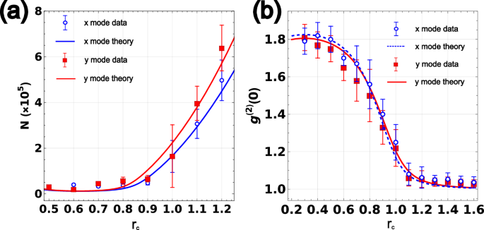
a The mean phonon number of the two modes as a function of the normalized modulation amplitude. The x and y modes have similar thresholds when they are parametrically driven. The solid lines are the theoretical fits and the error bar of each data point is the standard deviation of 50 measurements. b Normalized second-order phonon autocorrelation function at zero time delay, g(2)(0), as a function of normalized modulation amplitude, showing a phase transition of the two modes from thermal state to coherent state. The solid lines are the theoretical fits and the error bar of each data point is the standard deviation of 50 measurements.
The data presented in Figs. 2 and 3 define the essential characteristics of an optical tweezer phonon laser21. We emphasize that, in distinction to earlier single mode realizations21,22, our current two-mode implementation does not use linear amplification feedback to create phononic gain. Instead, the gain arises from the modulation of the coupling between the two modes and produces, above threshold, modes with coherence.
Next we turn to characterizing the useful and intriguing capability of two-mode squeezing as indicated by the system Hamiltonian of Eq. (2). While two-mode mechanical squeezing has been observed in other mechanical systems14,15,43 and single-mode squeezing has been observed for a levitated nanoparticle10,44, two-mode squeezing has never been observed in the latter system. Specifically, we investigate thermomechanical two-mode squeezing, which occurs when the mode coupling is driven at the sum frequency38,45. The normalized variances of the amplitude summation and difference, as a function of normalized driving modulation are presented in Fig. 4a. Here we are considering the variance of the summation of the amplitude (\(\overline{{\Delta }^{2}({r}_{x}+{r}_{y})}\) (represented by the purple line and data points) and the difference of the amplitude (\(\overline{{\Delta }^{2}({r}_{x}-{r}_{y})}\) (represented by the green line and data points); the overbars in the expressions indicate averages. At zero coupling, the variances of both the amplitude summation and difference are nearly identical, reflecting the independent nature of the x and y modes, as two distinct oscillation modes. When the sum frequency coupling is activated, the oscillations in the x and y modes are no longer independent, and the fluctuations of the oscillations in the two modes tend to correlate. As a result, the fluctuation of amplitude difference is reduced (as the fluctuations subtract), and the fluctuation of amplitude summation is amplified (as the noise in the two modes adds), and this behavior is maximized near the coupling threshold due to linear instability, where the whole system is at the boundary between the thermal and coherent behavior. When the system is above the threshold and the two modes are coherent, the fluctuation of the amplitude difference remains relatively unchanged, while the fluctuation of amplitude sum tends to decrease, approaching half the thermal variance as δ/δth → ∞, resulting in a reduction of the squeezing ratio45. The instability threshold in Fig. 4a is the same as the lasing threshold of Fig. 3, implying that our device combines, above threshold, the coherence and intensity of a laser with the low noise properties of a squeezed source. Note that we use the term ‘coherent state’ in the same sense as it is employed for an optical laser. The mode of such a device is often modeled by a pure Glauber coherent state, since g(2)(0) = 1, but it is in reality a statistical mixture of coherent states (due to the phase diffusion caused by the quantum noise of spontaneous emission) even in the absence of any technical noise46.
Fig. 4: Two-mode squeezing in a levitated nanoparticle.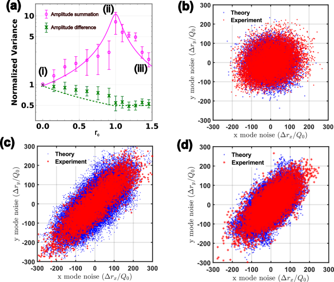
a The normalized variances of the two nanoparticle quadratures as a function of normalized modulation. The variance of the amplitude sum is presented by purple and that of the amplitude difference is presented by green. The fluctuation of the amplitude sum is amplified and that in the amplitude difference is squeezed when the coupling is increased from zero to below threshold. The variance of the amplitude sum decreases, while the variance of the amplitude difference stays at half of its original value, when the coupling is increased above the threshold. The solid and dashed lines are theoretical predictions found by solving the dynamical equations. The error bar of each data point represents the standard deviation. b–d are the scatter plots presenting the x and y mode amplitude noises at three different stages. The blue markers are the experimental data while the red markers are the theoretical expectation. b Scatter plots of x and y mode noises with no coupling, corresponding to the point (i) on (a), showing an almost symmetric disc shape in the two oscillation modes, and implying a squeezing ratio of 1, defined as the ratio of amplified variance to the squeezed variance. c Scatter plots of x and y mode noises with coupling strength around the threshold, corresponding to point (ii) on (a), showing squeezing in the diagonal direction and anti-squeezing in the anti-diagonal direction, with a squeezing ratio of 15.8 ± 0.8. d Scatter plots of x and y mode noises with coupling strength above the threshold, at point (iii) on (a), with the squeezing ratio 5.2 ± 0.6.
Theoretical predictions for the two-mode squeezing were made by solving the dynamical equations and considering the finite sampling time τm for measurements on the two-mode nanoparticle system (see Supplementary Note IV). In this way, the normalized variances of the amplified and squeezed states were found to be
$${\langle \delta {X}_{+}^{2}\rangle }_{{\tau }_{m}}^{{\phi }_{d}=0}=\frac{{\chi }_{-}}{{{{{\rm{r}}}}}_{c}-1}\,(\forall {{{{\rm{r}}}}}_{c})$$
(8)
$${\langle \delta {X}_{-}^{2}\rangle }_{{\tau }_{m}}^{{\phi }_{d}=0}=\frac{{\chi }_{+}}{{{{{\rm{r}}}}}_{c}+1}\,(0 < {{{{\rm{r}}}}}_{c} < 1)$$
(9)
$${\langle \delta {X}_{-}^{2}\rangle }_{{\tau }_{m}}^{{\phi }_{d}=0}=\frac{1}{2}\,({{{{\rm{r}}}}}_{c} > 1),$$
(10)
where \({\chi }_{\pm }=\,{{{\rm{sign}}}}\,({{{{\rm{r}}}}}_{c}\pm 1)-\frac{2}{\pi }\arctan \left[\frac{2\pi }{({{{{\rm{r}}}}}_{c}\pm 1){\gamma }_{0}{\tau }_{m}}\right]\) and \({\langle \delta {X}_{\pm }^{2}\rangle }_{{\tau }_{m}}^{{\phi }_{d}=0}\) are the variances of amplitude summation and difference in the two modes. The theoretical predictions align closely with the experimental data as illustrated in Fig. 4(a).
The x and y mode amplitude noise (Δrx and Δry), scaled by the oscillator length Q0, are plotted in Fig. 4b, c and d. Δrx and Δry are defined as the amplitude fluctuations relative to the mean amplitude of the two oscillation modes. The scatter plot of the x and y mode amplitude noise in the absence of mode-coupling [point (i) in Fig. 4(a)] is shown in Fig. 4b. Each point represents the oscillation amplitude deviation relative to the mean amplitude of a 0.5 ms time window in the x and y mode, red markers are experimental data and the blue markers are the results of simulating stochastic Langevin equations. Since the coupling is off, the two modes are not correlated, and the amplitude fluctuations in the two modes are nearly independent. When the coupling is around the threshold [point (ii) in Fig. 4a], the scatter plot between the two modes is squeezed in the diagonal direction and amplified in the anti-diagonal direction as shown in Fig. 4c, which indicates that the amplitude correlation between the two modes is maximized. As the coupling strength increases above the threshold [point (iii) in Fig. 4a], the scatter plot is illustrated in Fig. 4d, showing a reduced squeezing ratio, defined as the ratio of the variance of the amplitude summation to the variance of the amplitude difference.