
Continuum model of TBG
The schematic twist of graphene Brillouin zone and the consequent moiré Brillouin zone are drawn in Fig. 5. The length of the lattice vectors of mBZ is \(| {{{{\bf{G}}}}}_{1}|,| {{{{\bf{G}}}}}_{2}|=8\pi \sin (\Theta /2)/(3a)\) with a = 1.42 Å being the distance between the nearest carbon atoms. \({{{{\bf{K}}}}}_{1}^{\eta }\) and \({{{{\bf{K}}}}}_{2}^{\eta }\) are Dirac points of valley η = ± from the top (1) and bottom (2) layers, respectively. A momentum-space single-particle Hamiltonian, H0, considering intralayer hopping and interlayer hopping, can be constructed in the plane-wave basis as
$${H}_{0}= \sum\limits_{s,\eta,{{{\bf{k}}}},{{{\bf{G}}}},X,{{{{\bf{G}}}}}^{{\prime} },{X}^{{\prime} }}{d}_{s,\eta,{{{\bf{k}}}},{{{\bf{G}}}},X}^{{{\dagger}} }{H}_{{{{\bf{G}}}},X;{{{{\bf{G}}}}}^{{\prime} },{X}^{{\prime} }}^{s,\eta,{{{\bf{k}}}}}{d}_{s,\eta,{{{\bf{k}}}},{{{{\bf{G}}}}}^{{\prime} },{X}^{{\prime} }}\\= \sum\limits_{s,\eta,{{{\bf{k}}}}}{\vec{d}}_{s,\eta,{{{\bf{k}}}}}^{{{\dagger}} }{H}^{s,\eta,{{{\bf{k}}}}}{\vec{d}}_{s,\eta,{{{\bf{k}}}}}.$$
(6)
Here \({d}_{s,\eta,{{{\bf{k}}}},{{{\bf{G}}}},X}^{{{\dagger}} }\) is the creation operator for spin s, valley η, momentum k in mBZ, momentum folding G to account for the contributions from extended Brillouin zones, layer (1, 2) and sublattice (A, B), and \({\vec{d}}_{s,\eta,{{{\bf{k}}}}}^{{{\dagger}} }\) is the vector of \({d}_{s,\eta,{{{\bf{k}}}},{{{\bf{G}}}},X}^{{{\dagger}} }\). We use X ∈ {1A, 1B, 2A, 2B} to denote the layer and sublattice degrees of freedom. So, Hs,η,k is a matrix with the dimension of NGNX, which is actually the BM model7, and with the sub-blocks as
$$\begin{array}{l}{H}_{{{{\bf{G}}}},{{{{\bf{G}}}}}^{{\prime} }}^{s,\eta,{{{\bf{k}}}}} \hfill \\={\delta }_{{{{\bf{G}}}},{{{{\bf{G}}}}}^{{\prime} }}\hslash {v}_{{{{\rm{F}}}}}\left(\begin{array}{ll}-({{{\bf{k}}}}+{{{\bf{G}}}}-{{{{\bf{K}}}}}_{1}^{\eta })\cdot {\sigma }^{\eta }&0\\ 0&-({{{\bf{k}}}}+{{{\bf{G}}}}-{{{{\bf{K}}}}}_{2}^{\eta })\cdot {\sigma }^{\eta }\end{array}\right)\\+\left(\begin{array}{ll}0&{T}_{1}^{\eta }\\ {{T}_{2}^{\eta }}^{{{\dagger}} }&0\end{array}\right) \hfill \end{array}$$
(7)
with
$$\begin{array}{l}{T}_{l}^{\eta }=\left(\begin{array}{ll}{u}_{0}&{u}_{1}\\ {u}_{1}&{u}_{0}\end{array}\right){\delta }_{{{{\bf{G}}}},{{{{\bf{G}}}}}^{{\prime} }}+\left(\begin{array}{ll}{u}_{0}&{u}_{1}{{{{\rm{e}}}}}^{-i\frac{2\pi }{3}\eta }\\ {u}_{1}{{{{\rm{e}}}}}^{i\frac{2\pi }{3}\eta }&{u}_{0}\end{array}\right){\delta }_{{{{\bf{G}}}},{{{{\bf{G}}}}}^{{\prime} }+{(-1)}^{l}\eta {{{{\bf{G}}}}}_{1}}\\+\left(\begin{array}{ll}{u}_{0}&{u}_{1}{{{{\rm{e}}}}}^{i\frac{2\pi }{3}\eta }\\ {u}_{1}{{{{\rm{e}}}}}^{-i\frac{2\pi }{3}\eta }&{u}_{0}\end{array}\right){\delta }_{{{{\bf{G}}}},{{{{\bf{G}}}}}^{{\prime} }+{(-1)}^{l}\eta \left({{{{\bf{G}}}}}_{1}+{{{{\bf{G}}}}}_{2}\right)},\hfill \end{array}$$
(8)
where \({{{\bf{G}}}},{{{{\bf{G}}}}}^{{\prime} }\in \{{n}_{1}{{{{\bf{G}}}}}_{1}+{n}_{2}{{{{\bf{G}}}}}_{2}\}\) defining the lattices of mBZs, with n1 and n2 being integers, and a cutoff, ∣G∣, \(| {{{{\bf{G}}}}}^{{\prime} }| \le 6| {{{{\bf{G}}}}}_{1}|\), is applied. vF is the Fermi velocity and \(\hslash {v}_{{{{\rm{F}}}}}/(\sqrt{3}a)=2.37745\) eV. \({\sigma }^{\eta }=\left(\eta {\sigma }_{x},{\sigma }_{y}\right)\), where σx and σy are Pauli matrices in sublattice space. The first part of \({H}_{{{{\bf{G}}}},{{{{\bf{G}}}}}^{{\prime} }}^{s,\eta,{{{\bf{k}}}}}\) stands for intra-layer hopping of the top (1) layer and the bottom (2) layer, respectively, and the second part stands for inter-layer hopping u0 and u1, which are actually the moiré potentials.
Fig. 5: Momentum-space configuration of BZs and mBZs.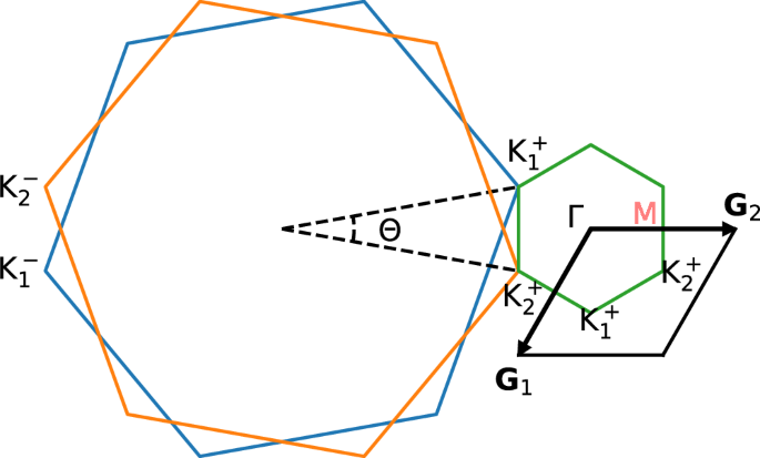
Twisting of graphene BZs as blue and orange hexagons leads to the mBZs as green hexagon or black rhombus with lattices of G1 and G2. Θ is the twist angle and \({{{{\bf{K}}}}}_{l}^{\eta }\) is a Dirac point of valley η and layer l. Γ and M are two high-symmetric points.
The dispersion of H0 for several twist angles are shown in Supplementary Fig. 2 with u0 = 60 meV, where enlarging of the bandwidth of two low-energy bands is seen with increasing Θ from MA, and the two low-energy bands are always isolated from the remote bands by ~ 60 meV. For the cases considered in this study, the minimum gap between low-energy bands and remote bands is not less than 20 meV while the maximum Coulomb potential is less than 6 meV, as shown in Supplementary Fig. 3. Thus, the low-energy physics can be well captured by these two low-energy bands.
The single-gated Coulomb interaction after Fouriers transformation is
$${H}_{{{{\rm{I}}}}}=\frac{1}{2\Omega }\sum \limits_{{{{\bf{q}}}}\in {{{\rm{mBZ}}}},{{{\bf{G}}}}}V({{{\bf{q}}}}+{{{\bf{G}}}})\delta {\rho }_{{{{\bf{q}}}}+{{{\bf{G}}}}}\delta {\rho }_{-{{{\bf{q}}}}-{{{\bf{G}}}}},$$
(9)
where
$$\begin{array}{l}\delta {\rho }_{{{{\bf{q}}}}+{{{\bf{G}}}}} \hfill \\=\sum\limits_{s,\eta,{{{\bf{k}}}},{{{{\bf{G}}}}}^{{\prime} },{X}^{{\prime} }}\left({d}_{s,\eta,{{{\bf{k}}}},{{{{\bf{G}}}}}^{{\prime} },{X}^{{\prime} }}^{{{\dagger}} }{d}_{s,\eta,{{{\bf{k}}}}+{{{\bf{q}}}}+{{{\bf{G}}}},{{{{\bf{G}}}}}^{{\prime} },{X}^{{\prime} }}-\frac{\nu+4}{8}{\delta }_{{{{\bf{q}}}},0}{\delta }_{{{{\bf{G}}}},0}\right)\\=\sum\limits_{s,\eta,{{{\bf{k}}}}}\left({\vec{d}}_{s,\eta,{{{\bf{k}}}}}^{{{\dagger}} }{\vec{d}}_{s,\eta,{{{\bf{k}}}}+{{{\bf{q}}}}+{{{\bf{G}}}}}-\frac{\nu+4}{8}{\delta }_{{{{\bf{q}}}},0}{\delta }_{{{{\bf{G}}}},0}\right).\hfill\end{array}$$
(10)
Here δρq+G is the electron density operator with respect to (ν + 4)/8 filling, and ν is the filling parameter with ν = 0 corresponding to the charge neutrality. \(\Omega=N| {{{{\bf{a}}}}}_{{{{\rm{M1}}}}}| | {{{{\bf{a}}}}}_{{{{\rm{M2}}}}}| \sqrt{3}/2\) is the total area of morié superlattice in real space, while aM1 and aM2 are the lattice vectors of the real-space unit cell of the superlattice with \(| {{{{\bf{a}}}}}_{{{{\rm{M1,M2}}}}}|=\sqrt{3}a/[2\sin (\Theta /2)]\). For the notational simplicity, from here on, q + G is denoted as \({{{\mathcal{Q}}}}\).
Denoting the eigenvalues and eigenvectors of the BM-model matrix Hs,η,k in Eq. (7) as \({\epsilon }_{{{{\bf{k}}}},m}^{s,\eta }\) and \(\left\vert {u}_{{{{\bf{k}}}},m}^{s,\eta }\right\rangle\), \({H}^{s,\eta,{{{\bf{k}}}}}\left\vert {u}_{{{{\bf{k}}}},m}^{s,\eta }\right\rangle={\epsilon }_{{{{\bf{k}}}},m}^{s,\eta }\left\vert {u}_{{{{\bf{k}}}},m}^{s,\eta }\right\rangle\), or
$${H}^{s,\eta,{{{\bf{k}}}}}{U}^{s,\eta,{{{\bf{k}}}}}={U}^{s,\eta,{{{\bf{k}}}}}{E}^{s,\eta,{{{\bf{k}}}}},$$
(11)
with each column of Us,η,k consisting of \(\left\vert {u}_{{{{\bf{k}}}},m}^{s,\eta }\right\rangle\) and Es,η,k is a diagonal matrix consisting of \({\epsilon }_{{{{\bf{k}}}},m}^{s,\eta }\), then H0 can be projected to the band basis as
$${H}_{0}= \sum\limits_{s,\eta,{{{\bf{k}}}}}{\vec{d}}_{s,\eta,{{{\bf{k}}}}}^{{{\dagger}} }{H}^{s,\eta,{{{\bf{k}}}}}{\vec{d}}_{s,\eta,{{{\bf{k}}}}}\\= \sum\limits_{s,\eta,{{{\bf{k}}}}}{\vec{d}}_{s,\eta,{{{\bf{k}}}}}^{{{\dagger}} }{U}^{s,\eta,{{{\bf{k}}}}}{{U}^{s,\eta,{{{\bf{k}}}}}}^{{{\dagger}} }{H}^{s,\eta,{{{\bf{k}}}}}{U}^{s,\eta,{{{\bf{k}}}}}{{U}^{s,\eta,{{{\bf{k}}}}}}^{{{\dagger}} }{\vec{d}}_{s,\eta,{{{\bf{k}}}}}\\= \sum\limits_{s,\eta,{{{\bf{k}}}}}{\vec{d}}_{s,\eta,{{{\bf{k}}}}}^{{{\dagger}} }{U}^{s,\eta,{{{\bf{k}}}}}{E}^{s,\eta,{{{\bf{k}}}}}{{U}^{s,\eta,{{{\bf{k}}}}}}^{{{\dagger}} }{\vec{d}}_{s,\eta,{{{\bf{k}}}}}.$$
(12)
Defining the projection
$${\vec{c}}_{s,\eta,{{{\bf{k}}}}}^{{{\dagger}} }={\vec{d}}_{s,\eta,{{{\bf{k}}}}}^{{{\dagger}} }{U}^{s,\eta,{{{\bf{k}}}}},$$
(13)
where \({\vec{c}}_{s,\eta,{{{\bf{k}}}}}\) is an operator vector with indices of G and X, with the element,
$${c}_{s,\eta,{{{\bf{k}}}},m}^{{{\dagger}} }=\sum\limits_{{{{\bf{G}}}},X}{d}_{s,\eta,{{{\bf{k}}}},{{{\bf{G}}}},X}^{{{\dagger}} }{\left| {u}_{{{{\bf{k}}}},m}^{s,\eta }\right\rangle }_{{{{\bf{G}}}},X},$$
(14)
then
$${H}_{0}= \sum\limits_{s,\eta,{{{\bf{k}}}}}{\vec{c}}_{s,\eta,{{{\bf{k}}}}}^{{{\dagger}} }{E}^{s,\eta,{{{\bf{k}}}}}{\vec{c}}_{s,\eta,{{{\bf{k}}}}}\\= \sum\limits_{s,\eta,{{{\bf{k}}}},m}{\epsilon }_{{{{\bf{k}}}},m}^{s,\eta }{c}_{s,\eta,{{{\bf{k}}}},m}^{{{\dagger}} }{c}_{s,\eta,{{{\bf{k}}}},m}.$$
(15)
This is the projection from the plane-wave basis, d†, to the band basis, c†. To make the projection to two low-energy bands, m relating to these two bands are kept.
Similarly, for the interaction,
$${\vec{d}}_{s,\eta,{{{\bf{k}}}}}^{{{\dagger}} }{\vec{d}}_{s,\eta,{{{\bf{k}}}}+{{{\mathcal{Q}}}}}= {\vec{d}}_{s,\eta,{{{\bf{k}}}}}^{{{\dagger}} }{U}_{{{{\bf{k}}}}}^{s,\eta }{{U}_{{{{\bf{k}}}}}^{s,\eta }}^{{{\dagger}} }{U}_{{{{\bf{k}}}}+{{{\mathcal{Q}}}}}^{s,\eta }{{U}_{{{{\bf{k}}}}+{{{\mathcal{Q}}}}}^{s,\eta }}^{{{\dagger}} }{\vec{d}}_{s,\eta,{{{\bf{k}}}}+{{{\mathcal{Q}}}}}\\= {\vec{c}}_{s,\eta,{{{\bf{k}}}}}^{{{\dagger}} }{{U}_{{{{\bf{k}}}}}^{s,\eta }}^{{{\dagger}} }{U}_{{{{\bf{k}}}}+{{{\mathcal{Q}}}}}^{s,\eta }{\vec{c}}_{s,\eta,{{{\bf{k}}}}+{{{\mathcal{Q}}}}}\\= \sum\limits_{m,n}{c}_{s,\eta,{{{\bf{k}}}},m}^{{{\dagger}} }{\left({{U}_{{{{\bf{k}}}}}^{s,\eta }}^{{{\dagger}} }{U}_{{{{\bf{k}}}}+{{{\mathcal{Q}}}}}^{s,\eta }\right)}_{m,n}{c}_{s,\eta,{{{\bf{k}}}}+{{{\mathcal{Q}}}},n}\\= \sum\limits_{m,n}{c}_{s,\eta,{{{\bf{k}}}},m}^{{{\dagger}} }{\lambda }_{m,n}^{s,\eta }({{{\bf{k}}}},{{{\mathcal{Q}}}}){c}_{s,\eta,{{{\bf{k}}}}+{{{\mathcal{Q}}}},n},$$
(16)
where the form factor is defined as
$$\begin{array}{rcl}{\lambda }_{m,n}^{s,\eta }({{{\bf{k}}}},{{{\mathcal{Q}}}})&=&{\left({{U}_{{{{\bf{k}}}}}^{s,\eta }}^{{{\dagger}} }{U}_{{{{\bf{k}}}}+{{{\mathcal{Q}}}}}^{s,\eta }\right)}_{m,n}\\ &=&\left\langle {u}_{{{{\bf{k}}}},m}^{s,\eta }| {u}_{{{{\bf{k}}}}+{{{\mathcal{Q}}}},n}^{s,\eta }\right\rangle .\end{array}$$
(17)
Note that we have made \({U}_{{{{\bf{k}}}}}^{s,\eta }={U}^{s,\eta,{{{\bf{k}}}}}\) to make the expressions compact. So,
$$\delta {\rho }_{{{{\mathcal{Q}}}}}=\sum\limits_{s,\eta,{{{\bf{k}}}}}\left(\sum\limits_{m,n}{\lambda }_{m,n}^{s,\eta }({{{\bf{k}}}},{{{\mathcal{Q}}}}){c}_{s,\eta,{{{\bf{k}}}},m}^{{{\dagger}} }{c}_{s,\eta,{{{\bf{k}}}}+{{{\mathcal{Q}}}},n}-\frac{\nu+4}{8}{\delta }_{{{{\bf{q}}}},0}{\delta }_{{{{\bf{G}}}},0}\right)$$
(18)
Moreover, since
$$\begin{array}{rcl}{\delta }_{{{{\bf{G}}}},0}&=&\sum\limits_{m}\left\langle {u}_{{{{\bf{k}}}},m}^{s,\eta }| {u}_{{{{\bf{k}}}}+{{{\bf{G}}}},m}^{s,\eta }\right\rangle \\ &=&\sum\limits_{m,n}{\lambda }_{m,n}^{s,\eta }({{{\bf{k}}}},{{{\bf{G}}}}){\delta }_{m,n},\end{array}$$
(19)
and further,
$${\delta }_{{{{\bf{q}}}},0}{\delta }_{{{{\bf{G}}}},0}=\sum\limits_{m,n}{\lambda }_{m,n}^{s,\eta }({{{\bf{k}}}},{{{\mathcal{Q}}}}){\delta }_{{{{\bf{q}}}},0}{\delta }_{m,n},$$
(20)
so that
$$\delta {\rho }_{{{{\mathcal{Q}}}}}=\sum\limits_{s,\eta,{{{\bf{k}}}},m,n}{\lambda }_{m,n}^{s,\eta }({{{\bf{k}}}},{{{\mathcal{Q}}}})\left({c}_{s,\eta,{{{\bf{k}}}},m}^{{{\dagger}} }{c}_{s,\eta,{{{\bf{k}}}}+{{{\mathcal{Q}}}},n}-\frac{\nu+4}{8}{\delta }_{{{{\bf{q}}}},0}{\delta }_{m,n}\right).$$
(21)
Since the set of \(\{| {{{\mathcal{Q}}}}| \ne 0\}\) is inversely symmetric, then
$${H}_{{{{\rm{I}}}}}= \sum\limits_{| {{{\mathcal{Q}}}}| \ne 0}\frac{1}{2\Omega }V({{{\mathcal{Q}}}})\delta {\rho }_{{{{\mathcal{Q}}}}}\delta {\rho }_{-{{{\mathcal{Q}}}}}\\= \sum\limits_{{{{\bf{Q}}}}}\frac{1}{2\Omega }V({{{\bf{Q}}}})(\delta {\rho }_{{{{\bf{Q}}}}}\delta {\rho }_{-{{{\bf{Q}}}}}+\delta {\rho }_{-{{{\bf{Q}}}}}\delta {\rho }_{{{{\bf{Q}}}}})\\= \sum\limits_{{{{\bf{Q}}}}}\frac{1}{4\Omega }V({{{\bf{Q}}}})\left({\left(\delta {\rho }_{-{{{\bf{Q}}}}}+\delta {\rho }_{{{{\bf{Q}}}}}\right)}^{2}-{\left(\delta {\rho }_{-{{{\bf{Q}}}}}-\delta {\rho }_{{{{\bf{Q}}}}}\right)}^{2}\right)\\= \sum\limits_{{{{\bf{Q}}}}}\frac{1}{4\Omega }V({{{\bf{Q}}}})\left({A}_{{{{\bf{Q}}}}}^{2}-{B}_{{{{\bf{Q}}}}}^{2}\right),$$
(22)
where the set of {Q} is any half of \(\{| {{{\mathcal{Q}}}}| \ne 0\}\). H0 in Eq. (15) and HI in Eq. (22) are exactly the terms used in the Hamiltonian (1) in the main text.
The KIVC order parameter is defined in the plane-wave basis as
$${O}_{{{{\rm{KIVC}}}}}({{{\bf{q}}}})\equiv \sum\limits_{s,{{{\bf{k}}}}}{\vec{d}}_{s,{{{\bf{k}}}}+{{{\bf{q}}}}}^{{{\dagger}} }{\eta }_{x}{\mu }_{y}{\sigma }_{x}{\vec{d}}_{s,{{{\bf{k}}}}}\\= \sum\limits_{s,\eta,{{{\bf{k}}}}}{\vec{d}}_{s,\eta,{{{\bf{k}}}}+{{{\bf{q}}}}}^{{{\dagger}} }{\mu }_{y}{\sigma }_{x}{\vec{d}}_{s,-\eta,{{{\bf{k}}}}},$$
(23)
and likewise projected to the band basis as
$${O}_{{{{\rm{KIVC}}}}}({{{\bf{q}}}})\\= \sum\limits_{s,\eta,{{{\bf{k}}}}}{\vec{d}}_{s,\eta,{{{\bf{k}}}}+{{{\bf{q}}}}}^{{{\dagger}} }{U}_{{{{\bf{k}}}}+{{{\bf{q}}}}}^{s,\eta }{{U}_{{{{\bf{k}}}}+{{{\bf{q}}}}}^{s,\eta }}^{{{\dagger}} }{\mu }_{y}{\sigma }_{x}{U}_{{{{\bf{k}}}}}^{s,-\eta }{{U}_{{{{\bf{k}}}}}^{s,-\eta }}^{{{\dagger}} }{\vec{d}}_{s,-\eta,{{{\bf{k}}}}}\\= \sum\limits_{s,\eta,{{{\bf{k}}}}}{\vec{c}}_{s,\eta,{{{\bf{k}}}}+{{{\bf{q}}}}}^{{{\dagger}} }{{U}_{{{{\bf{k}}}}+{{{\bf{q}}}}}^{s,\eta }}^{{{\dagger}} }{\mu }_{y}{\sigma }_{x}{U}_{{{{\bf{k}}}}}^{s,-\eta }{\vec{c}}_{s,-\eta,{{{\bf{k}}}}}\\= \sum\limits_{s,\eta,{{{\bf{k}}}},m,n}{c}_{s,\eta,{{{\bf{k}}}}+{{{\bf{q}}}},m}^{{{\dagger}} }{\left({{U}_{{{{\bf{k}}}}+{{{\bf{q}}}}}^{s,\eta }}^{{{\dagger}} }{\mu }_{y}{\sigma }_{x}{U}_{{{{\bf{k}}}}}^{s,-\eta }\right)}_{m,n}{c}_{s,-\eta,{{{\bf{k}}}},n}\\= \sum\limits_{s,\eta,{{{\bf{k}}}},m,n}{c}_{s,\eta,{{{\bf{k}}}}+{{{\bf{q}}}},m}^{{{\dagger}} }\langle {u}_{{{{\bf{k}}}}+{{{\bf{q}}}},m}^{s,\eta }| {\mu }_{y}{\sigma }_{x}| {u}_{{{{\bf{k}}}},n}^{s,-\eta }\rangle {c}_{s,-\eta,{{{\bf{k}}}},n}.$$
(24)
Similarly, the VP order parameter from the plane-wave basis to the band basis is
$${O}_{{{{\rm{VP}}}}}({{{\bf{q}}}}) \equiv \sum\limits_{s,{{{\bf{k}}}}}{\vec{d}}_{s,{{{\bf{k}}}}+{{{\bf{q}}}}}^{{{\dagger}} }{\eta }_{z}{\mu }_{0}{\sigma }_{0}{\vec{d}}_{s,{{{\bf{k}}}}}\\= -\sum\limits_{s,\eta,{{{\bf{k}}}},m,n}\eta {c}_{s,\eta,{{{\bf{k}}}}+{{{\bf{q}}}},m}^{{{\dagger}} }\langle {u}_{{{{\bf{k}}}}+{{{\bf{q}}}},m}^{s,\eta }| {\mu }_{0}{\sigma }_{0}| {u}_{{{{\bf{k}}}},n}^{s,\eta }\rangle {c}_{s,\eta,{{{\bf{k}}}},n}\\= -\sum\limits_{s,\eta,{{{\bf{k}}}},m,n}\eta {c}_{s,\eta,{{{\bf{k}}}}+{{{\bf{q}}}},m}^{{{\dagger}} }\langle {u}_{{{{\bf{k}}}}+{{{\bf{q}}}},m}^{s,\eta }| {u}_{{{{\bf{k}}}},n}^{s,\eta }\rangle {c}_{s,\eta,{{{\bf{k}}}},n}.$$
(25)
Gauge fixing
As can be seen from Eqs. (12), (16), the projections from the plane-wave basis to the band basis are gauge-independent within each spin-valley flavor, so that it is unnecessary to fix gauges within each spin-valley flavor. For different valleys, we fix \({{{\mathcal{PT}}}}\), which is ηxμyσx in plane-wave basis or ηyny in the band basis with ny acting on bands. \({{{\mathcal{PT}}}}\) leads to a complex conjugate between valleys.
In addition, to use the periodic condition, cs,η,k+G,m = cs,η,k,m, we impose
$${\left\vert {u}_{{{{\bf{k}}}}+{{{\bf{G}}}},m}^{s,\eta }\right\rangle }_{{{{{\bf{G}}}}}^{{\prime} },X}={\left\vert {u}_{{{{\bf{k}}}},m}^{s,\eta }\right\rangle }_{{{{{\bf{G}}}}}^{{\prime} }-{{{\bf{G}}}},X}.$$
(26)
The CFMC algorithm
The Hamiltonian in Eq. (1) has been solved with momentum-space QMC method with discretized auxiliary fields38,39. Similar to other determinantal QMC methods, it applies the Hubbard-Stratonovich transformation to decouple the Coulomb interaction, following the Trotter decomposition127,128,129,130,131. Due to \({{{\mathcal{PT}}}}\) symmetry, the system at charge neutrality is free of sign problem38,39. The simulation temperature is set to be 1/T ~ L with T = 0.5 meV for L = 6.
Original version of the momentum-space QMC method38,42 uses the discrete version of the Hubbard-Stratonovich transformation following a Trotter decomposition:
$$\exp \left(-{\alpha }_{1}({{{\bf{Q}}}}){A}_{{{{\bf{Q}}}}}^{2}\right)= \frac{1}{4}\sum\limits_{{l}_{{{{\bf{Q}}}},1}}\gamma \left({l}_{{{{\bf{Q}}}},1}\right)\exp \left({{{\rm{i}}}}\xi \left({l}_{{{{\bf{Q}}}},1}\right)\sqrt{{\alpha }_{1}({{{\bf{Q}}}})}{A}_{{{{\bf{Q}}}}}\right)\\ +{{{\mathcal{O}}}}\left({{\alpha }_{1}({{{\bf{Q}}}})}^{4}\right),$$
(27)
and
$$\exp \left({\alpha }_{1}({{{\bf{Q}}}}){B}_{{{{\bf{Q}}}}}^{2}\right)= \frac{1}{4}\sum\limits_{{l}_{{{{\bf{Q}}}},2}}\gamma \left({l}_{{{{\bf{Q}}}},2}\right)\exp \left(\xi \left({l}_{{{{\bf{Q}}}},2}\right)\sqrt{{\alpha }_{1}({{{\bf{Q}}}})}{B}_{{{{\bf{Q}}}}}\right)\\ +{{{\mathcal{O}}}}\left({{\alpha }_{1}({{{\bf{Q}}}})}^{4}\right).$$
(28)
Here lQ,1(2) = ± 1, ± 2 is a discrete auxiliary field, and the coeficients, \(\gamma (\pm 1)=1+\sqrt{6}/3\), \(\gamma (\pm 2)=1-\sqrt{6}/3\), \(\xi (\pm 1)=\pm \sqrt{6-2\sqrt{6}}\), and \(\xi (\pm 2)=\pm \sqrt{6+2\sqrt{6}}\) are taken from the eighth-order approximation as in 129. α1(Q) = ΔτV(Q)/4Ω < 8 × 10⁻³ with the imaginary time β = 1/(kBT) evenly sliced into Nτ pieces, as Δτ = β/Nτ. The partition function, \(Z={{{\rm{Tr}}}}\{\exp \left(-\beta H\right)\}\), yields
$$Z={\sum}_{\{{l}_{\tau,{{{\bf{Q}}}},1},{l}_{\tau,{{{\bf{Q}}}},2}\}}{{{\rm{Tr}}}}\,\{{U}_{C}\}$$
(29)
with
$${U}_{C}= {\prod }_{\tau=\bigtriangleup \tau }^{\beta }\exp \left(-\bigtriangleup \tau {H}_{0}\right)\prod\limits_{{{{\bf{Q}}}}}\frac{1}{16}\gamma \left({l}_{\tau,{{{\bf{Q}}}},1}\right)\gamma \left({l}_{\tau,Q,2}\right)\\ \times \exp \left({{{\rm{i}}}}\xi \left({l}_{\tau,{{{\bf{Q}}}},1}\right)\sqrt{{\alpha }_{1}({{{\bf{Q}}}})}{A}_{{{{\bf{Q}}}}}\right)\\ \times \exp \left(\xi \left({l}_{\tau,{{{\bf{Q}}}},2}\right)\sqrt{{\alpha }_{1}({{{\bf{Q}}}})}{B}_{{{{\bf{Q}}}}}\right)\\ +{{{\mathcal{O}}}}(8\times 1{0}^{-3}),$$
(30)
where C stands for a configuration of the auxiliary fields, and \({{{\mathcal{O}}}}(8\times 1{0}^{-3})\) stands for an error less than 8 × 10⁻³, which is usually 5 × 10⁻³, of the exact value.
With the partition function at hand, measurements can be done by sampling the discrete auxiliary fields with the Metropolis-Hastings scheme. Local update of one auxiliary field lQ,1(2) yields an acceptance rate around 0.4, and cluster update of multiple fields yields a vanishing acceptance rate. Each local update of a field lτ,Q,1(2) leads to the computation of matrix determinant with the complexity \({{{\mathcal{O}}}}({N}^{3})\), due to that AQ or BQ is non-diagonal. Combining with the absence of the efficient cluster update scheme for discrete fields, it leads to an overall complexity of at least \({{{\mathcal{O}}}}(\beta {N}^{4})\) in the original momentum-space QMC for a sweep to update 2NτNQ fields. Note that the number of the combinations (Q, 1(2)) is 2NQ ≈ 3N (the cutoff at ∣G1∣ makes the number of momentum exchanges roughly 3 times of the number of k points in mBZ). Therefore, the previous studies on TBG by QMC were heavily constrained by the accessible system sizes, with the largest one being L = 939,42.
To reduce the computational complexity, we develop a continuous-field Monte Carlo (CFMC) scheme to carry out cluster updates of multiple auxiliary fields at once. First of all, we switch to continuous auxiliary fields using the Gaussian integrals
$${{{{\rm{e}}}}}^{\frac{1}{2}{\alpha }_{2}{A}^{2}}=\frac{1}{\sqrt{2\pi }}\int_{-\infty }^{\infty }d\phi {{{{\rm{e}}}}}^{-\frac{1}{2}{\phi }^{2}}{{{{\rm{e}}}}}^{-\phi \sqrt{{\alpha }_{2}}A},$$
(31)
to rewrite the partition function of Eq. (29) in the form
$$Z= \int\left(\prod\limits_{\tau,{{{\bf{Q}}}}}d{\phi }_{\tau,{{{\bf{Q}}}},1}d{\phi }_{\tau,{{{\bf{Q}}}},2}\right){{{{\rm{e}}}}}^{-\frac{1}{2}\sum\limits_{\tau,Q}\left({\phi }_{\tau,{{{\bf{Q}}}},1}^{2}+{\phi }_{\tau,{{{\bf{Q}}}},2}^{2}\right)}\\ \times {{{\rm{Tr}}}}\left(\prod\limits_{\tau }{{{{\rm{e}}}}}^{{{{\rm{i}}}}\sum\limits_{{{{\bf{Q}}}}}\left(-{\phi }_{\tau,{{{\bf{Q}}}},1}\sqrt{{\alpha }_{2}({{{\bf{Q}}}})}{A}_{{{{\bf{Q}}}}}+{{{\rm{i}}}}{\phi }_{\tau,{{{\bf{Q}}}},2}\sqrt{{\alpha }_{2}({{{\bf{Q}}}})}{B}_{{{{\bf{Q}}}}}\right)}{{{{\rm{e}}}}}^{-\bigtriangleup \tau {H}_{0}}\right)\\ +{{{\mathcal{O}}}}(8\times 1{0}^{-3}),$$
(32)
where α2(Q) = ΔτV(Q)/2Ω. Note that the Gaussian decoupling is exact, so that the error of Z here comes from the Trotter decomposition, same as in Eq. (29).
We employ the same Metropolis-Hastings scheme for the updates of the continuous fields ϕτ,Q,1(2). Small updates of ϕτ,Q,1(2) would make an acceptance rate around one, while large updates would lead to a vanishing acceptance rate. The changes of ϕτ,Q,1(2), Δϕτ,Q,1(2), can be proposed from a Gaussian distribution or from the Hamiltonian’s dynamics.
Gaussian update scheme
For the Gaussian proposal, we tune the magnitudes of Δϕτ,Q,1(2) to make the acceptance rate around 0.4. The difference between the new and the old value of the auxiliary field is written as Δϕτ,Q,1(2) = rx with r being the control parameter to tune the magnitudes of Δϕτ,Q,1(2) and x generated from a standard normal distribution, \({{{\mathcal{N}}}}(0,1)\). The r is updated by r → r + (Ra − 0.4)Δr where Δr is a positive constant and Ra is the measured acceptance rate. Ra smaller than 0.4 means Δϕτ,Q,1(2) are larger than the desirable ones, and thus r is decreased, and vice versa. Ra ~ 0.4 should be achieved before the Markov process reaches equilibrium distribution.
All ϕτ,Q,1(2) of a specific imaginary time τ, with the number of ≈ 3N in total, are updated each time. Thus, only one calculation of matrix determinant with complexity \({{{\mathcal{O}}}}({N}^{3})\) is needed for each imaginary time τ.
The full protocol of CFMC with Gaussian proposals can be described as follows
1.
Generating all ϕτ,Q,1(2) fields using normal distribution \({{{\mathcal{N}}}}(0,1)\) and the current value of r parameter (initially we set r and Δr to 0.1).
2.
Updating all ϕτ,Q,1(2) of τ = β by Δϕτ,Q,1(2) = rx and accept-rejecting the update according to the Metropolis-Hastings scheme.
3.
Repeating the updates for all time slices from β to Δτ, then reversely to complete a full sweep, in the process of which Ra is calculated. After each sweep altering r using the rule r → r + (Ra − 0.4)Δr.
4.
Repeating the sweep until sufficient statistics is gained for all observables.
Hamiltonian update scheme
Since the auxiliary fields are continuous, it is easy to adopt more sophisticated updating schemes like Hamiltonian dynamics to improve the proposed Δϕτ,Q,1(2). This approach can significantly boost the acceptance rate, even for large global updates—a key feature of the so-called Hybrid Monte Carlo (HMC) algorithm, which has been successfully applied in condensed matter systems, especially those with long-range Coulomb interactions 132.
The partition function in Eq. (32) can be further expressed as
$$Z= \int\left(\prod\limits_{i}d{\phi }_{i}d{p}_{i}\right){{{{\rm{e}}}}}^{-\frac{1}{2}{\sum }_{i}\left({\phi }_{i}^{2}+{p}_{i}^{2}\right)}\det \left({{{\rm{I}}}}+{B}_{C}(\beta,0)\right)\\ +{{{\mathcal{O}}}}(8\times 1{0}^{-3}),$$
(33)
where the index i ≡ (τ, Q, m) with m = 1, 2 is employed for compactness and an artificial momentum pi is introduced for ϕi. Moreover,
$$ \det \left({{{\rm{I}}}}+{B}_{C}(\beta,0)\right)=\\ \quad {{{\rm{Tr}}}}\left(\prod\limits_{\tau }{{{{\rm{e}}}}}^{{{{\rm{i}}}}{\sum }_{{{{\bf{Q}}}}}\left(-{\phi }_{\tau,{{{\bf{Q}}}},1}\sqrt{{\alpha }_{2}({{{\bf{Q}}}})}{A}_{{{{\bf{Q}}}}}+{{{\rm{i}}}}{\phi }_{\tau,{{{\bf{Q}}}},2}\sqrt{{\alpha }_{2}({{{\bf{Q}}}})}{B}_{{{{\bf{Q}}}}}\right)}{{{{\rm{e}}}}}^{-\bigtriangleup \tau {H}_{0}}\right),$$
(34)
which is nonnegative for charge-neutral TBG. Furthermore, the partition function can be expressed as
$$Z=\int\left(\prod\limits_{i}d{\phi }_{i}d{p}_{i}\right){{{{\rm{e}}}}}^{-{{{\mathcal{H}}}}}+{{{\mathcal{O}}}}(8\times 1{0}^{-3}),$$
(35)
with the effective Hamiltonian
$${{{\mathcal{H}}}}\equiv \frac{1}{2}{\sum}_{i}\left({\phi }_{i}^{2}+{p}_{i}^{2}\right)-\ln \left(\det \left({{{\rm{I}}}}+{B}_{C}(\beta,0)\right)\right).$$
(36)
The Hamiltonian dynamics is applied as
$$\frac{d{p}_{i}}{dt}= -\frac{\partial {{{\mathcal{H}}}}}{\partial {\phi }_{i}}\\= -{\phi }_{i}+4{{{\rm{Tr}}}}\left({J}_{{{{\bf{Q}}}}}({{{\rm{I}}}}-G(\tau ))\right)+{{{\mathcal{O}}}}(1{0}^{-2})\\ \frac{d{\phi }_{i}}{dt}= \frac{\partial {{{\mathcal{H}}}}}{\partial {p}_{i}}\\= {p}_{i},$$
(37)
where G(τ) is the equal-time Green’s function for s = ↑ and η = + , and JQ is the matrix form of AQ or BQ for m = 1 or 2. The Hamiltonian dynamics facilitates the increased acceptance rates through the conservation of the Hamiltonian along equal-energy trajectories.
The outperformance of the CFMC algorithm
The comparison of performances of CFMC and discretized-field QMC (DQMC) algorithms is shown in Fig. 6 using the same physical settings. It can be clearly seen that CFMC indeed reduces the computational complexity from O(βN4) to O(βN3), as the system size increases.
Fig. 6: Computational complexities of DQMC and CFMC with the same physical settings.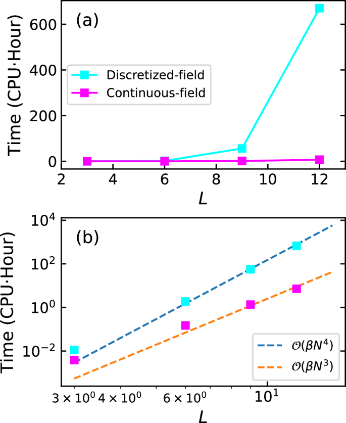
We measure the CPU time consumed by the two methods for 100 sweeps in the units of CPU core hours, and show the time in a linear-linear scale (a) and a log-log scale (b). Note that inverse temperature also sclaes with the systems size: β ~ L. The data can be very well described by the fits of βN4 and βN3 with N = L × L for DQMC and CFMC, respectively, especially in the limit of large system sizes.
The CPU time per update is not the only metric which defines the performance of the Monte Carlo scheme. It can be that different updates lead to substantially different distributions of the observables (despite the average values being fixed)133. Thus, the faster algorithm can potentially suffer from larger statistical fluctuations, which can even cancel the gain in the speed of update. In order to check this, we plot the Monte Carlo time series of an IVC structure factor from DQMC and CFMC simlations. Results for Θ = 1.08°, 1. 2°, and 1. 3° are shown in Supplementary Fig. 6. The histograms for the time series are drawn on top of them using the red and blue lines, respectively. The overlap of histograms indicates that fluctuations of DQMC and CFMC are very similar, thus the overall increase in performance from O(βN4) scaling to O(βN3) sclaing still holds.
The autocorrelations for the CFMC and DQMC methods are also compared, as illustrated in Supplementary Fig. 7. Since the measurements are done after the updates of the fields in each time slice, we compare autocorrelation for measurements separated by a Euclidean time interval Δt. The autocorrelation time is indeed larger for CFMC, which offsets the factor of N in speedup in simulations at MA and at the smallest lattice size. However, since the autocorrelation time does not depend on the lattice size, moving away from L = 6 and Θ = 1.08° reveals a greater advantage: the difference in scaling (O(βN4) for DQMC versus O(βN3) for CFMC) quickly outweighs the impact of the increased autocorrelation time (see the concrete examples in the caption of the Supplementary Fig. 7. We therefore conclude that CFMC significantly enhances the performances of the Monte Carlo simulations.
Stochastic analytic continuation
The stochastic analytic continuation (SAC)41,42,43,44,85,86,134 method is also employed to extract the real frequency spectral functions. The Green’s function relates to the real frequency spectral function as 42
$$G({{{\bf{k}}}},\tau )=\int_{-\infty }^{\infty }d\omega \left(\frac{{{{{\rm{e}}}}}^{-\omega \tau }}{1+{{{{\rm{e}}}}}^{-\beta \omega }}\right)A({{{\bf{k}}}},\omega ).$$
(38)
A variational ansatz of A(k, ω) simulating an annealing process is applied. For each momentum k, \(A({{{\bf{k}}}},\omega )={\sum }_{i=1}^{{N}_{\omega }}{A}_{i}\delta (\omega -{\omega }_{i})\) where frequencies ωi initially form regular grid with length of 0.5kBT of Nω = 4000 points symmetrically distributed around 0. Then A(k, ω) is estimated by sampling over the grid of ωi, using Eq. (38) and the effective action
$${\chi }^{2}= {\sum}_{{\tau }_{1},{\tau }_{2}}\left(\overline{G}({\tau }_{1})-\int_{-\infty }^{\infty }d\omega \left(\frac{{{{{\rm{e}}}}}^{-\omega \tau }}{1+{{{{\rm{e}}}}}^{-\beta \omega }}\right)A(\omega )\right){({C}^{-1})}_{{\tau }_{1},{\tau }_{2}}\\ \times \left(\overline{G}({\tau }_{2})-\int_{-\infty }^{\infty }d\omega \left(\frac{{{{{\rm{e}}}}}^{-\omega \tau }}{1+{{{{\rm{e}}}}}^{-\beta \omega }}\right)A(\omega )\right),$$
(39)
where
$$\begin{array}{l}{C}_{{\tau }_{1},{\tau }_{2}}\\=\frac{1}{{N}_{b}({N}_{b}-1)}{\sum }_{b=1}^{{N}_{b}}\left({G}^{b}({\tau }_{1})-\overline{G}({\tau }_{1})\right)\left({G}^{b}({\tau }_{2})-\overline{G}({\tau }_{2})\right),\end{array}$$
(40)
with τ1 and τ2 referring to selected imaginary times where the errors of Green’s functions are less than 0.1. Gb(τ1,2) is the Green’s function of b-th bin at τ1,2, and \(\overline{G}({\tau }_{1,2})\) is the average of Gb(τ1,2) over all bins. Importance sampling of Metropolis-Hastings type is employed, and the sampling weight is \(W=\exp \left(-{\chi }^{2}/(2{T}_{1})\right)\) where T1 is the artificial temperature, which decreases from 5 by a factor of 0.6 in each step. The final value of T1 is defined by the average effective action satisfying the relation\(\langle {\chi }^{2}\rangle={\chi }_{\min }^{2}+2\sqrt{{\chi }_{\min }^{2}}\)42, and this final value of T1 is used to obtain the spectra.
Computation of the free energy
The free energy is difficult to obtain numerically, since exponentially large or small numbers are usually involved. Let us denote the partition function as Z = ∑CWCPC, where WC corresponds to the bosonic part of the action and PC corresponds to the fermionic determinant. Since the kinetic energy is included as \({{{{\rm{e}}}}}^{-\bigtriangleup \tau {H}_{0}}\) in Eq. (32), PC becomes exponentially large as the kinetic energy grows with twist angle (see Supplementary Fig. 2). One might think that positive and negative terms in the matrix \({{{{\rm{e}}}}}^{-\bigtriangleup \tau {H}_{0}}\) form pairs, so that they cancel each other and the magnitude of PC does not change a lot with the twist angle. However, the identity matrix in the relation, \({{{\rm{Tr}}}}\left({{{{\rm{e}}}}}^{{\sum }_{i,j}{c}_{i}^{{{\dagger}} }{A}_{i,j}{c}_{j}}{{{{\rm{e}}}}}^{{\sum }_{i,j}{c}_{i}^{{{\dagger}} }{B}_{i,j}{c}_{j}}\right)=\det \left({{{\rm{I}}}}+{{{{\rm{e}}}}}^{A}{{{{\rm{e}}}}}^{B}\right)\), forbids this cancellation.
The free energy F can be theoretically measured by
$$F \equiv -\frac{1}{\beta }\ln (Z)\\= -\frac{1}{\beta }\ln \left(\sum\limits_{C}{W}_{C}{P}_{C}\right)\\= -\frac{1}{\beta }\ln \left(\left(\sum\limits_{C}{W}_{C}\right)\frac{{\sum }_{C}{W}_{C}{P}_{C}}{{\sum }_{C}{W}_{C}}\right)\\= -\frac{1}{\beta }\ln \left(\sum\limits_{C}{W}_{C}\right)-\frac{1}{\beta }\ln \left(\frac{{\sum }_{C}{W}_{C}{P}_{C}}{{\sum }_{C}{W}_{C}}\right),$$
(41)
which simply means the importance sampling of PC over the weight defined by WC. However, PC is exponentially large in our case, so that direct sampling of a moderate-size system is inaccessible.
Recently, an integral algorithm to efficiently sample exponential observables such as free energy and entanglement entropy was developed 87. Dumping the constant number \(-\ln \left({\sum }_{C}{W}_{C}\right)/\beta\) for a specific T, we can rewrite F as
$$F=-\frac{1}{\beta }\int_{0}^{1}dt\frac{\partial \ln (f(t))}{\partial t},$$
(42)
if \(f(1)=\left({\sum }_{C}{W}_{C}{P}_{C}\right)/\left({\sum }_{C}{W}_{C}\right)\) and f(0) = 1. Subsequently, we define f(t) as f(t) = 〈etX〉, so that \(\langle {{{{\rm{e}}}}}^{X}\rangle=\left({\sum }_{C}{W}_{C}{P}_{C}\right)/\left({\sum }_{C}{W}_{C}\right)\) and \(X=\ln (P)\). Substituting it in (42), we get
$$F= -\frac{1}{\beta }\int_{0}^{1}dt\frac{\langle X{{{{\rm{e}}}}}^{tX}\rangle }{\langle {{{{\rm{e}}}}}^{tX}\rangle }\\= -\frac{1}{\beta }\int_{0}^{1}dt\frac{{\sum }_{C}{W}_{C}{P}_{C}^{t}\ln ({P}_{C})}{{\sum }_{C}{W}_{C}{P}_{C}^{t}}.$$
(43)
Thus, the exponentially large values of observables are avoided and we need only the importance samplings of \(\ln ({P}_{C})\) over the weight of \({W}_{C}{P}_{C}^{t}\).
Padé approximants and scaling exponents
The critical exponents characterize a particular universality class and depend on the dimensionality, symmetry and the relevant degrees of freedom. The transition to the KIVC order in TBG falls in the universality classe of the chiral XY GN model. This was considered previously via perturbative renormalization up to four-loop order in an ϵ expansion54, where ϵ is the deviation from the the upper critical spacetime dimension D = 4 − ϵ of the model In ref. 54, a scale dependence is introduced in the fields ϕ and ψ, as well as for the mass term m, quartic coupling λ, and Yukawa coupling g from Eq. (3), and their renormalization is calculated. Based on this, the inverse correlation-length exponent ν−1, the correction-to-scaling exponent ω, the fermion and the boson anomlous dimension ηψ, ηϕ are determined and their expression for general fermion flavor number Nf is provided up to fourth order in ϵ. We use these results and apply them to our case of interest, the KIVC-DSM transition in TBG. To obtain an estimate for the critical exponents for the case of (2+1) dimensions, we calculate the different Padé approximant
$${P}_{[m/n]}(\epsilon )=\frac{{a}_{0}+{a}_{1}\epsilon+\cdots+{a}_{m}{\epsilon }^{m}}{1+{b}_{1}\epsilon+\cdots+{b}_{n}{\epsilon }^{n}}$$
(44)
for a general fermion flavor number Nf for the exponents ν−1, ηϕ. Selecting only those that do not exhibit any singularities or poles, which in our case are P[2/2](ϵ) and P[3/1](ϵ), we obtain the numerical values for Nf = 16 and ϵ = 1 and use the hyperscaling relation to determine the order parameter exponent β, β = ν(D − 2 + ηϕ)/2. We subsequently average over these values and based on those provide the numerical uncertainties.