
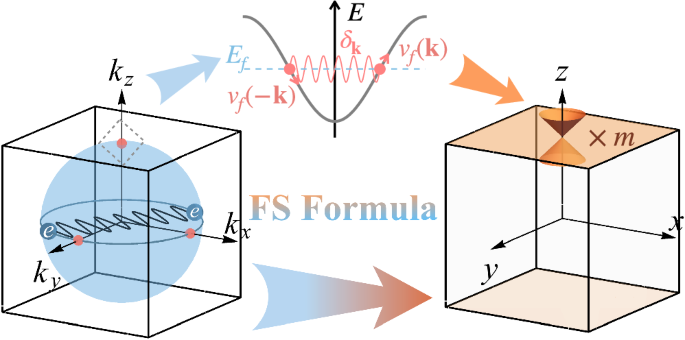
Fermi surface formulas
In this work, we focus on s-wave-like pairing symmetries, formally defined by the symmetry properties of the order parameter Δk. Let Uk(g) be a representation of a space group symmetry g. We say that the pairing symmetry is s-wave-like if \({U}_{{{\bf{k}}}}(g){\Delta }_{{{\bf{k}}}}{U}_{-{{\bf{k}}}}^{\top }(g)={\Delta }_{g{{\bf{k}}}}\) for all symmetries in a given space group. It should be noted that the s-wave-like pairing symmetry does not necessarily mean that the system is a conventional s-wave superconductor. For example, consider a single orbital superconducting order Δk = (d(k) ⋅ σ)iσy under the mirror symmetry \({{{\mathcal{M}}}}_{z}\) along the z-axis, where \({{\bf{d}}}({{\bf{k}}})=(0,{{\mathrm{i}}}\sin {k}_{x},0)\) and σi=0,x,y,z are Pauli matrices in spin space. While this is p-wave like, the pairing symmetry is s-wave like, as one can see \({{\rm{i}}}{\upsigma }_{z}{\Delta }_{{{\bf{k}}}}{({{\rm{i}}}{\upsigma }_{z})}^{\top }={\Delta }_{{{{\mathcal{M}}}}_{z}{{\bf{k}}}}\). Another representative example is s±-wave pairing.
Topological invariants are often defined on subregions in momentum space. For convenience, we decompose the Brillouin zone into points, line segments, and polygons in a symmetric manner68,69. See Fig. 2(b) for an illustration of the decomposition. We assign an orientation to each component. For example, line segment a in Fig. 2(b) is oriented from Γ to X. In this work, we consider topological invariants defined on the line segments.
Fig. 2: Illustration of the model (10) and (11).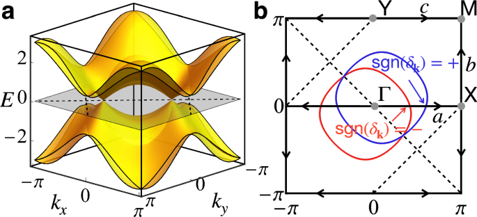 The alternative text for this image may have been generated using AI.
a shows the energy dispersion of the BdG Hamiltonian (11). b shows decomposition of the Brillouin zone, Fermi surfaces (colored solid lines), and the pairing nodes (dashed lines). The solid black lines and arrows denote the line segments specified by the gray endpoints and their orientations. The red and blue colors in the figure indicate Fermi surfaces with mirror eigenvalues + i and − i, respectively. The intersections of the Fermi surface and the pairing nodes correspond to the gapless points in (a). The parameters are set to be {t, λ, μ, Δ} = { − 1, 0.3, − 1, 0.3}.
Before presenting our main results on the Fermi surfaces of the topological invariants, we introduce our basic assumptions on target systems. We always assume that superconductors are in the weak coupling regime. More precisely, we assume that the target superconducting system can be continuously deformed into a superconductor that possesses the following properties:
(i)
intraband pairings dominate, i.e., all interband pairings are negligible;
(ii)
the superconducting gap is negligible except on Fermi surfaces.
In addition, we further assume that the following conditions are satisfied:
(iii)
all Fermi surfaces are minimally degenerate as allowed by symmetries;
(iv)
normal state energies at high-symmetry points are not at the Fermi level;
(v)
there is no superconducting node on all line segments, including their endpoints.
The assumptions (iii) and (iv) usually hold for realistic systems. The assumption (v) must be satisfied to define topological invariants on line segments.
Under these five assumptions, intraband pairing potentials and Fermi velocities can determine the values of topological invariants defined on the line segments. To define intraband pairing potentials and Fermi velocities, we consider the m-th Fermi point at km and momenta k in its neighborhood. Let \({\Phi }_{{{\bf{k}}},m}^{\alpha }\) be a matrix whose columns are eigenvectors of the normal conducting Hamiltonian hk with the energy \({\varepsilon }_{{{\bf{k}}},m}^{\alpha }\), where α is a label of an irreducible representation (irrep) \({u}_{{{\bf{k}}}}^{\alpha }(g)\). In other words, \({\Phi }_{{{\bf{k}}},m}^{\alpha }\) satisfies the relations \({h}_{{{\bf{k}}}}{\Phi }_{{{\bf{k}}},m}^{\alpha }={\varepsilon }_{{{\bf{k}}},m}^{\alpha }{\Phi }_{{{\bf{k}}},m}^{\alpha }\) and \({U}_{{{\bf{k}}}}(g){\Phi }_{{{\bf{k}}},m}^{\alpha }={\Phi }_{{{\bf{k}}},m}^{\alpha }{u}_{{{\bf{k}}}}^{\alpha }(g)\). Then, the intraband pairing potential is defined by a projected superconducting order
$${\tilde{\Delta }}_{{{\bf{k}}},m}^{\alpha } := {[{\Phi }_{{{\bf{k}}},m}^{\alpha }]}^{{\dagger} }{\Delta }_{{{\bf{k}}}}{[U({{\mathcal{T}}})]}^{*}{\Phi }_{{{\bf{k}}},m}^{\alpha }.$$
(1)
Here, \(U({{\mathcal{T}}})\) is a unitary representation of time-reversal symmetry (TRS) satisfying \(U({{\mathcal{T}}}){[U({{\mathcal{T}}})]}^{*}=-{\mathbb{1}}\), where \({\mathbb{1}}\) is the identity matrix. The above intraband pairing satisfies the relations
$${[{\tilde{\Delta }}_{{{\bf{k}}},m}^{\alpha }]}^{{\dagger} }={\tilde{\Delta }}_{{{\bf{k}}},m}^{\alpha };\,\,{u}_{{{\bf{k}}}}^{\alpha }(g){\tilde{\Delta }}_{{{\bf{k}}},m}^{\alpha }{[{u}_{{{\bf{k}}}}^{\alpha }(g)]}^{{\dagger} }={\tilde{\Delta }}_{{{\bf{k}}},m}^{\alpha }.$$
(2)
Since \({u}_{{{\bf{k}}}}^{\alpha }(g)\) is irreducible, the intraband pairing is proportional to the identity matrix. In particular, when we consider the Fermi point km on the line segment l, we represent \({\tilde{\Delta }}_{{{{\bf{k}}}}_{m},m}^{\alpha }\) by
$${\tilde{\Delta }}_{{{{\bf{k}}}}_{m},m}^{\alpha }={\delta }_{m}^{(l,\alpha )}{\mathbb{1}}\,\,\,({\delta }_{m}^{(l,\alpha )}\in {\mathbb{R}}),$$
(3)
where \({\delta }_{m}^{(l,\alpha )}\) represents the intraband pairing potential at the m-th Fermi point with irrep α on line segment l.
The Fermi velocity is defined by the directional derivative of the energy. Suppose that we consider a line segment l connecting from kA to kB, and that the m-th Fermi point at km lies on this line segment. The Fermi velocity of the energy \({\varepsilon }_{{{\bf{k}}},m}^{\alpha }\) is given by
$${v}_{m}^{(l,\alpha )} := {{{\boldsymbol{\nabla }}}}_{{{\bf{k}}}}{\varepsilon }_{{{\bf{k}}},m}^{\alpha }{| }_{{{\bf{k}}}={{{\bf{k}}}}_{m}}\cdot {\hat{{{\bf{e}}}}}_{l},$$
(4)
where \({\hat{{{\bf{e}}}}}_{l}=({{{\bf{k}}}}_{{\mathrm{B}}}-{{{\bf{k}}}}_{{\mathrm{A}}})/\parallel {{{\bf{k}}}}_{{\mathrm{B}}}-{{{\bf{k}}}}_{{\mathrm{A}}}\parallel\).
Based on these two quantities, we define a set of integer-valued quantities \({\{{{{\mathcal{N}}}}_{(l,\alpha )}\}}_{l,\alpha }\) for a given system:
$${{{\mathcal{N}}}}_{(l,\alpha )} := {\sum }_{m=1}^{{n}_{(l,\alpha )}}\,{{\mathrm{sgn}}}({v}_{m}^{(l,\alpha )})\frac{1-{{\mathrm{sgn}}}\,({\delta }_{m}^{(l,\alpha )})}{2}\in {\mathbb{Z}},$$
(5)
where n(l, α) is the number of minimally degenerate Fermi points with irrep α on line segment l. In fact, this integer-valued quantity encodes the topological nature of superconducting phases under the above assumptions.
Now, we are ready to provide concrete forms of Fermi-surface formulas of topological invariants. For each space group, there exist three types of topological invariants: (i) \({\mathbb{Z}}\)-valued invariants \({\{{{{\mathcal{W}}}}_{i}^{\rm gapless}\}}_{i=1}^{{N}_{\rm gapless}}\) to detect gapless points in two-dimensional subregions surrounded by line segments; (ii) \({\mathbb{Z}}\)-valued invariants \({\{{{{\mathcal{W}}}}_{i}^{\rm gapped}\}}_{i=1}^{{N}_{\rm gapped}}\) to capture gapped topological phases; (iii) \({{\mathbb{Z}}}_{\lambda }\)-valued invariants \({\{{{{\mathcal{X}}}}_{i}\}}_{i=1}^{M}\) to identify gapped topological phases. It should be emphasized that both the number of defined topological invariants (Ngapless, Ngapped, M), and topological invariants themselves depend on a given space group. Notably, gapped topological phases detected by \({\{{{{\mathcal{W}}}}_{i}^{\rm gapped}\}}_{i=1}^{{N}_{\rm gapped}}\) and \({\{{{{\mathcal{X}}}}_{i}\}}_{i=1}^{M}\) must have protected gapless surface states. Furthermore, \({\{{{{\mathcal{W}}}}_{i}^{\rm gapless}\}}_{i=1}^{{N}_{\rm gapless}}\) can detect all stable gapless phases in all space groups with s-wave-like pairing symmetries (See Supplementary Note 2 for more details).
Our Fermi-surface formulas of these invariants are given by
$${{{\mathcal{W}}}}_{i}^{\rm gapless}= {\sum }_{l,\alpha }{w}_{i,(l,\alpha )}^{\rm gapless}{{{\mathcal{N}}}}_{(l,\alpha )}\\= {\sum }_{l,\alpha }{w}_{i,(l,\alpha )}^{\rm gapless}{\sum }_{m=1}^{{n}_{(l,\alpha )}}\,{{\mathrm{sgn}}}({v}_{m}^{(l,\alpha )})\frac{1-{{\mathrm{sgn}}}\,{({\delta }_{m}^{(l,\alpha )})}}{2},$$
(6)
$${{{\mathcal{W}}}}_{i}^{\rm gapped}= {\sum }_{l,\alpha }{w}_{i,(l,\alpha )}^{\rm gapped}{{{\mathcal{N}}}}_{(l,\alpha )}\\= {\sum }_{l,\alpha }{w}_{i,(l,\alpha )}^{\rm gapped}{\sum }_{m=1}^{{n}_{(l,\alpha )}}\,{{\mathrm{sgn}}}({v}_{m}^{(l,\alpha )})\frac{1-{{\mathrm{sgn}}}\,{({\delta }_{m}^{(l,\alpha )})}}{2},$$
(7)
$${{{\mathcal{X}}}}_{i}= {\sum }_{l,\alpha }{x}_{i,(l,\alpha )}{{{\mathcal{N}}}}_{(l,\alpha )}\,\,{{\mathrm{mod}}}\,\lambda \\= {\sum }_{l,\alpha }{x}_{i,(l,\alpha )}{\sum }_{m=1}^{{n}_{(l,\alpha )}}\,{{\mathrm{sgn}}}({v}_{m}^{(l,\alpha )})\frac{1-{{\mathrm{sgn}}}\,({\delta }_{m}^{(l,\alpha )})}{2}\,\,{{\mathrm{mod}}}\,\lambda,$$
(8)
where \({w}_{i,(l,\alpha )}^{\rm gapless},{w}_{i,(l,\alpha )}^{\rm gapped},{x}_{i,(l,\alpha )}\in {\mathbb{Z}}\) represent contribution weights of irrep α on line segment l for topological invariants. In other words, these integer-valued quantities tell us about two important things: which line segments and irreps are relevant for topological invariants, and how we should combine Fermi-point data \({\{{{{\mathcal{N}}}}_{(l,\alpha )}\}}_{l,\alpha }\) to detect the topological nature of superconducting phases. For a given space group, we can systematically determine these contribution weights by Atiyah-Hirzebruch spectral sequence. See ref. 46 for more details. For \({{\mathbb{Z}}}_{2}\)-valued invariants, we can drop \(\,{{\mathrm{sgn}}}\,({v}_{m}^{(l,\alpha )})\) since n = − n mod 2 for an integer n. As a result, the formulas can be further simplified to
$${{{\mathcal{X}}}}_{i}={\sum }_{l,\alpha }{x}_{i,(l,\alpha )}{\sum }_{m=1}^{{n}_{(l,\alpha )}}\frac{1-\,{{\mathrm{sgn}}}\,({\delta }_{m}^{(l,\alpha )})}{2}\,\,{{\mathrm{mod}}}\,\,2.$$
(9)
These formulas immediately give us the following insight. The quantities (6)–(9) are always trivial for superconductors whose intraband pairings have the same sign everywhere. This means that superconductors in the BCS limit, which can be connected to the vacuum without closing gap, cannot have nontrivial values of Eqs. (6)–(9).
We make three remarks on our formulas. First, our Fermi-surface formulas are well-defined for a given decomposition, including the orientations of line segments, of the Brillouin zone in a space group. In Supplementary Information, we provide our formulas together with all line segments we used for all layer groups and space groups. If we adopt a different decomposition, we may have physically equivalent but different forms of the formulas. This is because changing the decomposition can change the contribution weights in general. Next, topological invariants for gapped phases, \({\{{{{\mathcal{W}}}}_{i}^{\rm {gapped}}\}}_{i=1}^{{N}_{\rm {gapped}}}\) and \({\{{{{\mathcal{X}}}}_{i}\}}_{i=1}^{M}\), are meaningful only when invariants for gapless points, \({\{{{{\mathcal{W}}}}_{i}^{\rm {gapless}}\}}_{i=1}^{{N}_{\rm {gapless}}}\), are all trivial. Lastly, topological invariants defined on higher-dimensional subspaces would be required for gapped topological phases that cannot be detected by our formulas. For example, detecting the nonzero three-dimensional winding number \({w}_{3{{\rm{D}}}}\in {\mathbb{Z}}\) requires information on the entire three-dimensional Brillouin zone70. Nonetheless, our Fermi surface formula can still detect \({w}_{3{{\rm{D}}}}\,{{\mathrm{mod}}}\,\,n\) (where n depends on the space group), as seen below. This is similar to the situation for symmetry indicators57,58,71.
Examples
Here, we demonstrate how it works through three theoretical models constructed by the real-space construction method and one realistic model from real material.
First, we consider a quasi-two-dimensional gapless superconductor in the layer group p11m. This layer group is generated by the mirror symmetry \({{\mathcal{M}}}_{z}=\{{M}_{z}|(000)\}\) and translation symmetries along x- and y-direction. The decomposition of the Brillouin zone is shown in Fig. 2(b). The normal state Hamiltonian for the superconductor is
$${h}_{{{\bf{k}}}}=t(\cos {k}_{x}+\cos {k}_{y}){s}_{0}+\lambda (\sin {k}_{x}+\sin {k}_{y}){s}_{3},$$
(10)
and the corresponding BdG Hamiltonian takes the form
$${H}_{{{\bf{k}}}}^{\rm {BdG}}=[{h}_{{{\bf{k}}}}-\mu ]{\kappa }_{3}+{\Delta }_{\rm {sc}}(\sin {k}_{x}+\sin {k}_{y}){s}_{1}{\kappa }_{1},$$
(11)
where the Pauli matrices sj and κj (j = 0, 1, 2, 3) stand for spins and the Nambu spinor. In addition to TRS and mirror symmetry \({{{\mathcal{M}}}}_{z}\), the BdG Hamiltonian inherently possesses particle-hole symmetry \({{\mathcal{C}}}\). For the above BdG Hamiltonian, their representations are given by
$${U}^{\rm {BdG}}({{\mathcal{T}}})={{\rm{i}}}{s}_{2},\,{U}^{\rm {BdG}}({{\mathcal{C}}})={\kappa }_{1},\,{U}^{\rm {BdG}}({{{\mathcal{M}}}}_{z})={{\rm{i}}}{\kappa }_{3}{s}_{3}.$$
(12)
The pairing term \({\Delta }_{{{\bf{k}}}}={\Delta }_{{{\rm{sc}}}}(\sin {k}_{x}+\sin {k}_{y}){s}_{1}\) remains invariant under mirror symmetry \({{{\mathcal{M}}}}_{z}\): \({U}_{{{\bf{k}}}}({{{\mathcal{M}}}}_{z}){\Delta }_{{{\bf{k}}}}{U}_{{{\bf{k}}}}^{{{\top }}}=\Delta_{{{{\mathcal{M}}}}_{z}{\bf{k}}}\), where \({U}_{{{\bf{k}}}}({{M}}_{z})\) is the representation of the mirror symmetry in the normal phase. Therefore, the pairing exhibits the s-wave-like pairing symmetry. As shown in Fig. 2(a), the energy spectrum of \({H}_{{{\bf{k}}}}^{\rm {BdG}}\)(11) has two superconducting gapless points.
Our formula for \({\mathbb{Z}}\)-valued invariants can detect these gapless points. Using Eq. (6), we find the formula
$${{{\mathcal{W}}}}_{1}^{\rm gapless}= {\sum }_{\alpha=\pm }\alpha \,\left[{\sum }_{m=1}^{{n}_{(c,\alpha )}}\,{{\mathrm{sgn}}}({v}_{m}^{(c,\alpha )})\frac{1-{{\mathrm{sgn}}}\,({\delta }_{m}^{(c,\alpha )})}{2} \right. \\ \left. -{\sum }_{m=1}^{{n}_{(a,\alpha )}}\,{{\mathrm{sgn}}}({v}_{m}^{(a,\alpha )})\frac{1-{{\mathrm{sgn}}}\,({\delta }_{m}^{(a,\alpha )})}{2}\right],$$
(13)
where α = ± means the mirror eigenvalue ± i for eigenstates of the normal state Hamiltonian (10). The signs of Fermi velocities v(a, ±) on the line segment a are positive. According to the sign of δk shown in Fig. 2(b), we have \({{{\mathcal{W}}}}^{\rm {gapless}}=-1\). In fact, the invariant is equivalent to the mirror winding number defined on a loop ( − π, 0) → (π, 0) → (π, π) → ( − π, π) → ( − π, 0). The nontrivial mirror winding number indicates the existence of gapless points inside the loop72.
Next, we consider a gapped topological superconductor (TSC) in layer group p21/b11 to show that our formulas can be used even when the formula in ref. 70 cannot. Generators of this layer group are glide symmetry \({{{\mathcal{G}}}}_{x}=\{{M}_{x}| (\frac{1}{2}\frac{1}{2}0)\}\), inversion symmetry \({{\mathcal{I}}}=\{I| (000)\}\), and translation symmetry along x-direction. In the presence of inversion symmetry and TRS, Fermi surfaces in spinful electronic systems must be at least twofold degenerate. Furthermore, topological invariants for class DIII in the tenfold classification73,74,75 are also trivial for even-parity pairings. Therefore, this symmetry setting is out of the scope of ref. 70.
Here, we describe our model in which there are four sublattice degrees of freedom labeled by (τz, σz) = ( ± 1, ± 1). Their coordinates in a unit cell are specified by \((x,y)=\frac{1}{4}[(2-{\tau }_{z})(1,0)+(1-{\sigma }_{z})(0,1)]\) [see Fig. 3(a)]. According to ref. 45, the classification of gapped topological phases is \({{\mathbb{Z}}}_{2}\), whose generator is constructed by placing one-dimensional TSCs along x = 1/4 and x = 3/4 in each unit cell. To realize this, we consider a model whose normal state Hamiltonian is given by
$${h}_{{{\bf{k}}}}=t({\Gamma }_{010}+\cos {k}_{y}{\Gamma }_{010}+\sin {k}_{y}{\Gamma }_{020}),$$
(14)
and the BdG Hamiltonian is
$${H}_{{{\bf{k}}}}^{\rm {BdG}}=[{h}_{{{\bf{k}}}}-\mu ]{\kappa }_{3}+2{\Delta }_{{\mathrm{sc}}}\sin {k}_{y}{\Gamma }_{301}{\kappa }_{1},$$
(15)
where Γijk:= τi ⊗ σj ⊗ sk(i, j, k = 0, 1, 2, 3). As mentioned above, the minimal degeneracy of states is twofold at each momentum. However, the Fermi surfaces of hk in Eq. (14) are fourfold degenerate, which violates assumption (iii), as indicated by the gray dashed lines in Fig. 3(b). This violation can be easily resolved by introducing symmetry-allowed perturbations that are small enough not to change any topology, as shown by the solid gray lines in Fig. 3(b).
Fig. 3: Illustration of the model in layer group p21/b11.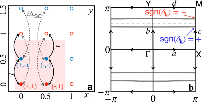 The alternative text for this image may have been generated using AI.
a Real-space description of the model. The red shaded region indicates the unit cell. The red and blue solid circles denote the four sublattices labeled by (τz, σz) = ( ± 1, ± 1) in the unit cell. The solid (dashed) arrows represent the hopping between the sublattice degrees in the normal (pairing) part of the BdG Hamiltonian (15). b Fermi surfaces for the Hamiltonian (14). The gray solid (dashed) lines show the normal-state Fermi surfaces with (without) symmetry-allowed perturbations. The red and blue colors mean states with glide eigenvalue \(+i{e}^{-i{k}_{y}/2}\) and \(-i{e}^{-i{k}_{y}/2}\), respectively. The parameters are set to be {t, μ} = { − 1, 1}.
The \({{\mathbb{Z}}}_{2}\) topology can be diagnosed by our formula for \({{\mathbb{Z}}}_{2}\)-valued invariant in Eq. (9). The decomposition of the Brillouin zone is shown in Fig. 3(b). Then, the formula is given by
$${{{\mathcal{X}}}}_{1}={\sum }_{\alpha=\pm }{\sum }_{m=1}^{{n}_{(c,\alpha )}}\frac{1-\,{{\mathrm{sgn}}}({\delta }_{m}^{(c,\alpha )})}{2}+{\sum }_{\beta=\pm }{\sum }_{m=1}^{{n}_{(d,\beta )}}\frac{1-{{\mathrm{sgn}}}\,({\delta }_{m}^{(d,\beta )})}{2},$$
(16)
where α = ± represents the glide eigenvalue \(\pm {{\rm{ie}}}^{-i{k}_{y}/2}\) on the line segment c, and β = ± denotes the screw symmetry \({{{\mathcal{S}}}}_{x}={{{\mathcal{G}}}}_{x}{{\mathcal{I}}}\) eigenvalue \(\pm {{\rm{ie}}}^{-i{k}_{x}/2}\) on the line segment d. According to the sign of δk shown in Fig. 3(b), we have \({{\mathcal{X}}}=1\) mod 2.
Last, we discuss a strong TSC in space group P41 to show that our formula can inform the three-dimensional winding number w3D modulo four. This space group is generated by fourfold screw symmetry \({{{\mathcal{S}}}}_{4z}=\{{C}_{4z}| (00\frac{1}{4})\}\) and translation symmetries along x- and y-directions.
Our model is described as follows. There are four sublattice degrees of freedom in a unit cell, whose coordinates in a unit cell are (x, y, z) = (0, 0, 0), (0, 0, 1/4), (0, 0, 1/2), and (0, 0, 3/4), labeled as 1, 2, 3, and 4, respectively. The normal state Hamiltonian is constructed as
$${\hat{{{\mathcal{H}}}}}_{0}= {\sum }_{s,{{\bf{R}}}}{\sum }_{i=1}^{4}-\frac{t}{2}({\hat{c}}_{si{{\bf{R}}}+{{\bf{a}}}}^{{\dagger} }{\hat{c}}_{si{{\bf{R}}}}+{\hat{c}}_{si{{\bf{R}}}+{{\bf{b}}}}^{{\dagger} }{\hat{c}}_{si{{\bf{R}}}})+h.c.\\ +{\sum }_{s,{{\bf{R}}}}-\frac{t}{2}({\hat{c}}_{s1{{\bf{R}}}}^{{\dagger} }{\hat{c}}_{s2{{\bf{R}}}}+{\hat{c}}_{s2{{\bf{R}}}}^{{\dagger} }{\hat{c}}_{s3{{\bf{R}}}}+{\hat{c}}_{s4{{\bf{R}}}}^{{\dagger} }{\hat{c}}_{s3{{\bf{R}}}})+h.c.\\ + {\sum }_{s,{{\bf{R}}}}-\frac{t}{2}{\hat{c}}_{s4{{\bf{R}}}+{{\bf{c}}}}^{{\dagger} }{\hat{c}}_{s1{{\bf{R}}}}+h.c.,{\sum }_{s,{{\bf{R}}},i}{\hat{c}}_{si{{\bf{R}}}+{{\bf{c}}}}^{{\dagger} }{\hat{c}}_{si{{\bf{R}}}},$$
(17)
where the \({\widehat{c}}_{si{{\bf{R}}}}\,({\widehat{c}}_{si{{\bf{R}}}}^{{\dagger} })\) is the annihilation (creation) operator of an electron at the i-th sublattice with spin s in the unit cell at R. Also, a, b, and c are the primitive lattice vectors along x-, y-, and z-direction, respectively. The pairing term is given by
$$\hat{\Delta }= {\sum }_{s,{{\bf{R}}}}-\frac{i}{2}{\Delta }_{{\mathrm{sc}}}({\hat{c}}_{s1{{\bf{R}}}}^{{\dagger} }{\hat{c}}_{\overline{s}2{{\bf{R}}}}^{{\dagger} }+{\hat{c}}_{s4{{\bf{R}}}}^{{\dagger} }{\hat{c}}_{\overline{s}3{{\bf{R}}}}^{{\dagger} }+{\hat{c}}_{s2{{\bf{R}}}}^{{\dagger} }{\hat{c}}_{\overline{s}3{{\bf{R}}}}^{{\dagger} })+h.c.\\ +{\sum }_{s,{{\bf{R}}}}\frac{i}{2}{\Delta }_{{\mathrm{sc}}}({\hat{c}}_{s1{{\bf{R}}}}^{{\dagger} }{\hat{c}}_{\overline{s}4{{\bf{R}}}+{{\bf{c}}}}^{{\dagger} }-{\sum }_{i=1}^{4}s{\hat{c}}_{si{{\bf{R}}}}^{{\dagger} }{\widehat{c}}_{si{{\bf{R}}}+{{\bf{a}}}}^{{\dagger} })+h.c.\\ +{\sum }_{s,{{\bf{R}}}}{\sum }_{i=1}^{4}\frac{1}{2}{\Delta }_{{\mathrm{sc}}}{\widehat{c}}_{si{{\bf{R}}}}^{{\dagger} }{\widehat{c}}_{si{{\bf{R}}}+{{\bf{b}}}}^{{\dagger} }-h.c.$$
(18)
with s and \(\overline{s}\) being the opposite spin. It is easy to check the system described by \({\hat{{{\mathcal{H}}}}}_{\rm BdG}={\hat{{{\mathcal{H}}}}}_{0}+\hat{\Delta }\) has the nonzero three-dimensional winding number w3D = 1.
Here, we compute the \({{\mathbb{Z}}}_{8}\)-valued invariant by our formula (8):
$${{{\mathcal{X}}}}_{3}= {\sum }_{l=e,g}{\sum }_{\alpha=1,3,5,7}(4-\alpha ){\sum }_{m=1}^{{n}_{(l,\alpha )}}\,{{\rm{sgn}}}({v}_{m}^{(l,\alpha )})\frac{1-{{\rm{sgn}}}\,({\delta }_{m}^{(l,\alpha )})}{2} \\ \, +{\sum }_{l=c,d}{\sum }_{m=1}^{{n}_{l}}\,{{\mathrm{sgn}}}\,({v}_{m}^{l})(1-\,{{\mathrm{sgn}}}\,({\delta }_{m}^{l}))\\ \, +{\sum }_{\beta=\pm }\beta {\sum }_{m=1}^{{n}_{(f,\beta )}}\,{{\mathrm{sgn}}}\,({v}_{m}^{(f,\beta )})(1-\,{{\mathrm{sgn}}}\,({\delta }_{m}^{(f,\beta )})),$$
(19)
where for line segment l = e and g, \({v}_{m}^{(l,\alpha )}\) and \({\delta }_{m}^{(l,\alpha )}\,(\alpha=1,3,5,7)\) are defined for screw eigenvalue \({e}^{-i(\alpha \pi+{k}_{z})/4}\); for line segment f, \({v}_{m}^{(f,\beta )}\) and \({\delta }_{m}^{(f,\beta )}\,(\beta=\pm )\) are defined for twofold rotation eigenvalues βi. After adding symmetry allowed perturbations to lift the accidental degeneracy in \({\hat{{{\mathcal{H}}}}}_{0}\), the energy spectrum is as shown in Fig. 4. According to the sign of δk shown in Fig. 4, we find \({{{\mathcal{X}}}}_{3}=3\). In Methods, we show that \({{{\mathcal{X}}}}_{3}\) mod 4 serves as a \({{\mathbb{Z}}}_{4}\)-valued indicator of w3D.
Fig. 4: The band structure of the model (17) with symmetry-allowed perturbations in space group P41.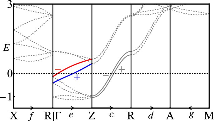 The alternative text for this image may have been generated using AI.
Solid lines (dashed lines) represent bands crossing (not crossing) the Fermi level. The arrows represent the positive direction of the line segments c, d, e, f, and g. The red and blue colors mean states with screw eigenvalue \({e}^{-i(3\pi+{k}_{z})/4}\) and \({e}^{-i(\pi+{k}_{z})/4}\), respectively. The + and − represent the sign of δk at the corresponding Fermi point. The parameters are set to be {t, μ} = {1, 1.8}.
Application to realistic materials
We discuss CaFeAs2, whose space group is P21, to demonstrate how to apply our formula to realistic materials based on first-principles calculations.
In Fig. 5, we show the band structure and Fermi surfaces obtained by DFT calculations. From the raw data of Fig. 5(a), we notice that there are eight Fermi surfaces around the Γ point and four Fermi surfaces around the M point. This implies that although the Fermi surfaces in Fig. 5(b) and (c) seem to be degenerate, there is no Fermi surface degeneracy. This is consistent with the symmetry analysis.
Fig. 5: First-principle calculation results for CaFeAs2.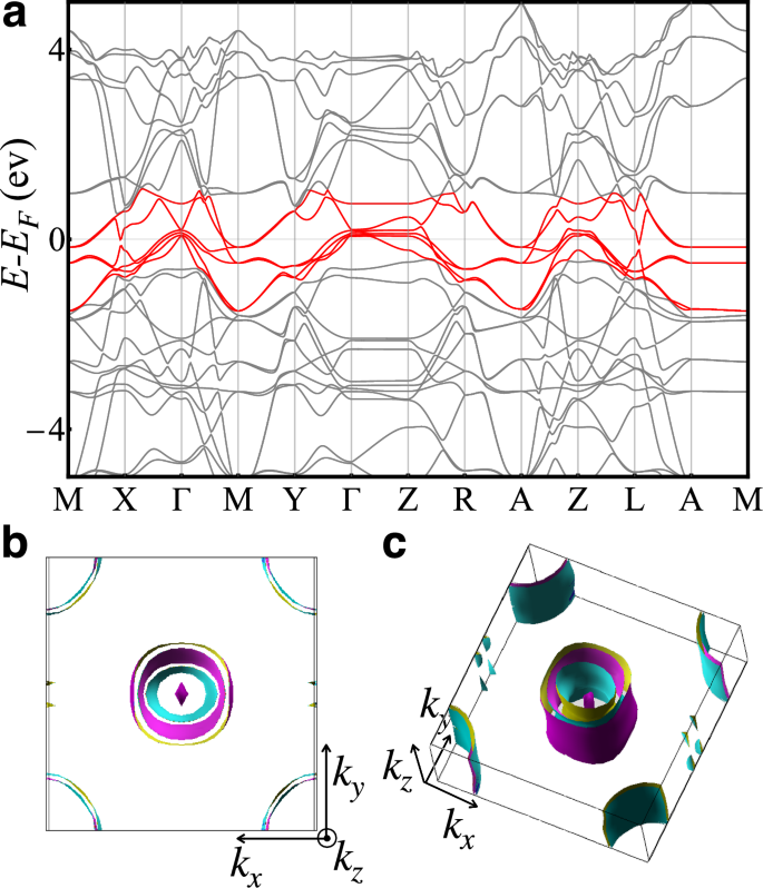 The alternative text for this image may have been generated using AI.
a The band structure of CaFeAs2. The bands near the Fermi energy EF are marked in red. M, X, Γ, Y, Z, R, A, L represent (π/2, π/2, 0), (π/2, 0, 0), (0, 0, 0), (0, π/2, 0), (0, 0, π/2), (0, π/2, π/2), (π/2, π/2, π/2), (π/2, 0, π/2) in the Brillouin zone, respectively. b, c The Fermi surface of CaFeAs2 with different viewpoints. The Fermi surfaces are visualized by XCrySDen87.
One can see that the kz-dependence of Fermi surfaces is sufficiently weak, and topological properties inherit the quasi-two-dimensional nature of its electronic structure. Therefore, we focus on kz = 0 plane with the exchange of kx- and ky-axes to illustrate the workflow of our diagnostic scheme, which results in Layer group p2111 (No. 9).
According to our Fermi surface formula, there exist a \({\mathbb{Z}}\)-valued invariant for gapless points, a \({{\mathbb{Z}}}_{2}\)-valued invariant, and a \({{\mathbb{Z}}}_{4}\)-valued invariant, whose expressions are given by
$${{{\mathcal{W}}}}_{1}^{\rm gapless}= {\sum }_{m=1}^{{n}_{{a}_{1}}}\,{{\mathrm{sgn}}}({v}_{m}^{{a}_{1}})\frac{1-{{\mathrm{sgn}}}({\delta }_{m}^{{a}_{1}})}{2}+{\sum }_{m=1}^{{n}_{{a}_{2}}}{{\mathrm{sgn}}}({v}_{m}^{{a}_{2}})\frac{1-{{\mathrm{sgn}}}({\delta }_{m}^{{a}_{2}})}{2}\\ -{\sum }_{m=1}^{{n}_{{b}_{1}}}{{\mathrm{sgn}}}({v}_{m}^{{b}_{1}})\frac{1-{{\mathrm{sgn}}}\,({\delta }_{m}^{{b}_{1}})}{2}+2{\sum }_{m=1}^{{n}_{{c}_{1}}}\,{{\mathrm{sgn}}}({v}_{m}^{{c}_{1}})\frac{1-{{\mathrm{sgn}}}({\delta }_{m}^{{c}_{1}})}{2}\\ -{\sum }_{m=1}^{{n}_{{d}_{1}}}sgn({v}_{m}^{{d}_{1}})\frac{1-{{\mathrm{sgn}}}({\delta }_{m}^{{d}_{1}})}{2}-{\sum }_{m=1}^{{n}_{{d}_{2}}}{{\mathrm{sgn}}}({v}_{m}^{{d}_{2}})\frac{1-{{\mathrm{sgn}}}\,({\delta }_{m}^{{d}_{2}})}{2};$$
(20)
$${{{\mathcal{X}}}}_{1}={\sum }_{m=1}^{{n}_{{b}_{1}}}\frac{1-\,{{\mathrm{sgn}}}({\delta }_{m}^{{b}_{1}})}{2}+{\sum }_{m=1}^{{n}_{{d}_{1}}}\frac{1-{{\mathrm{sgn}}}({\delta }_{m}^{{d}_{1}})}{2}+{\sum }_{m=1}^{{n}_{{d}_{2}}}\frac{1-{{\mathrm{sgn}}}\,({\delta }_{m}^{{d}_{2}})}{2}\,\,{{\mathrm{mod}}}\,\,2;$$
(21)
$${{{\mathcal{X}}}}_{2}= 2{\sum }_{m=1}^{{n}_{{a}_{2}}}\,{{\mathrm{sgn}}}({v}_{m}^{{a}_{2}})\frac{1-{{\mathrm{sgn}}}({\delta }_{m}^{{a}_{2}})}{2}-{\sum }_{m=1}^{{n}_{{b}_{1}}}{{\mathrm{sgn}}}({v}_{m}^{{b}_{1}})\frac{1-{{\mathrm{sgn}}}({\delta }_{m}^{{b}_{1}})}{2}\\ -2{\sum }_{m=1}^{{n}_{{d}_{1}}}{{\mathrm{sgn}}}({v}_{m}^{{d}_{1}})\frac{1-{{\mathrm{sgn}}}\,({\delta }_{m}^{{d}_{1}})}{2}\,\,{{\mathrm{mod}}}\,\,4.$$
(22)
Here, a1 and d1 (a2 and d2) are symbols of the irreducible representations whose character of screw symmetry along x-axis is \(-{{\rm{i}}}{e}^{-{{\rm{i}}}{k}_{x}/2}\,(+{{\rm{i}}}{e}^{-{{\rm{i}}}{k}_{x}/2})\) (see Section L9 in Supplementary Information for more detailed information).
As a demonstration, here we discuss some scenarios out of all possibilities, in which sign changes happen between the Fermi surfaces near the M point while fixing the pairing signs of the Fermi surfaces near the Γ point to be positive. Although a global gauge transformation can give rise to the global minus sign of the superconducting order parameter, this does not affect the topology. As a result, there are six inequivalent pairing sign choices for possible fully gapped superconducting states (whose \({{{\mathcal{W}}}}_{1}^{\rm {gapless}}\) must be trivial), as shown in Fig. 6(b–g). According to the formulas of the invariants, we find that four of these configurations correspond to topologically nontrivial states, \(({{{\mathcal{W}}}}_{1}^{\rm {gapless}},{{{\mathcal{X}}}}_{1},{{{\mathcal{X}}}}_{2})=(0,0,2)\). This phase is equivalent to x-direction stacking copies of one-dimensional class DIII topological superconductors along the y-direction, as shown in Fig. 6(h) (see Supplementary Note 3A for more details). The model in Fig. 6(h) with a small perturbation is a second-order topological superconductor with Majorana corner modes, as shown in Fig. 6(i).
Fig. 6: Demonstration of our diagnosis of topological phases based on first-principles calculation results.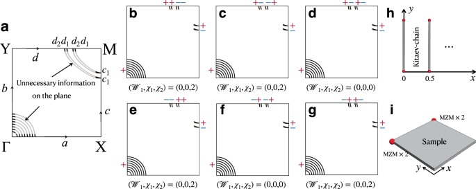 The alternative text for this image may have been generated using AI.
a Fermi surface of quasi-2D CaFeAs2 based on the DFT-calculated data. a, b, c, d are the one-cell, whose directions are labeled by arrows. ci and di represent the irreducible representations on the one-cell c and d. Γ, X, Y, M represent (0, 0), (π, 0), (0, π) and (π, π). b–g The six inequivalent pairing sign configurations satisfying \({{{\mathcal{W}}}}_{1}^{\rm {gapless}}=0\). + and − represent the pairing sign \({\delta }_{i}^{l}\) of i-th Fermi points on the line segment l. \({{\mathcal{W}}}\), \({{{\mathcal{X}}}}_{1}\) and \({{{\mathcal{X}}}}_{2}\) represent the value of the topological invariants defined in Eqs. (20), (21) and (22). h The real-space construction of the topological nontrivial state with \(({{\mathcal{W}}},{{{\mathcal{X}}}}_{1},{{{\mathcal{X}}}}_{2})=(0,0,2)\). i The corner modes of the topological nontrivial state with \(({{\mathcal{W}}},{{{\mathcal{X}}}}_{1},{{{\mathcal{X}}}}_{2})=(0,0,2)\).
Finally, let us return to the discussion of the three-dimensional nature. Due to its quasi-two-dimensional electronic nature, three-dimensional topological properties can be understood by stacking the aforementioned two-dimensional topological states along the z-direction. As a result, we conclude that this three-dimensional topological phase exhibits hinge modes along the z-direction.