
This section outlines details and specifications of the benchmark metrics, tasks, and baselines.
Algorithm track metrics
NeuroBench includes correctness and complexity metrics, the latter of which is divided in static and workload metrics. Static metrics do not depend on the model inference and input data, while the workload metrics do. Note that the defined metrics reflect only the model and model execution. Data pre-processors and post-processors are not taken into account in the v1.0 algorithm track results.
Footprint
The footprint metric reflects the memory footprint a model. It is distinct from execution memory, which may incur further usage, e.g. to store activations. It is computed for a model by accumulating the sizes of the model’s parameters and buffers, in bytes. Parameters store the model synaptic weights, and buffers include other inference memory requirements, such as the internal states of recurrent or spiking layers and buffers of recent input data, if the model must record data for input binning. Considering n parameters, each requiring pi bytes, and b buffers of size qj, the total model footprint is \({\sum }_{i=0}^{n}{p}_{i}+\mathop{\sum }_{j=0}^{b}{q}_{j}\).
Model execution rate
Execution rate is a numeric which is not directly computed by the harness, but should be reported by the user. The numeric reflects the real-time correlation of the rate at which the model computes input data. If the model processes input with a temporal stride of t seconds, then the rate should be reported as t−1 Hz. Note the distinction between stride and bin window – input can be binned in overlapping windows, but execution rate depends on the temporal stride of window processing. As an example, a model may use 50 ms windows of input and compute every 10 ms, which would give an execution rate of 100 Hz.
This numeric is currently not well-defined for models operating under event-based or continuous-time contexts. These limitations will be addressed in future benchmark versions.
Connection sparsity
The parameter matrices of each layer l in a model, representing synaptic weights, are collected, and the number of zero weights ml and total weights nl are aggregated, with the connection sparsity defined as \(\frac{{\sum }_{l}{m}_{l}}{{\sum }_{l}{n}_{l}}\).
Activation sparsity
Activation sparsity is computed after the inference phase. The sparsity is calculated by accumulating the number of zero activations (z), over all neuron layers (l), timesteps (t), and input samples (i) and dividing by the total number of neurons (N), \(\frac{{\sum }_{l}{\sum }_{t}{\sum }_{i}{z}_{l,t}^{i}}{{\sum }_{t}{\sum }_{l}{\sum }_{i}{N}_{l,t}^{i}}\). The outputs of ReLU functions and spikes from spiking neurons are considered activations.
Synaptic operations
Synaptic operations are the multiplication of weights by activation or input data, and are calculated using the inputs and weights of connection layers (e.g., torch.nn.Linear and torch.nn.Conv2d). Effective synaptic operations are operations where a non-zero weight is multiplied by a non-zero activation. Effective operations are further divided into multiply-accumulates (MACs), and accumulates (ACs), where accumulates correlate with activations or input data only containing values of [−1, 0, 1], and multiply-accumulates cover all other cases. The reported number of synaptic operations is the average number of synaptic operations required per model execution, the rate of which is defined by the model execution rate metric.
The number of effective synaptic operations is computed by performing the forward pass of a layer and counting the number of operations in which there is no zero multiplication. Practically, this is implemented in the harness by setting all non-zero weights in the layer and all the non-zero activations to 1, then performing the forward pass and summing the output to give the number of synaptic operations.
The number of dense synaptic operations is computed in a similar fashion, by setting all weights and activations to 1 and accumulating the output of the forward pass. Biases are not taken into account in the calculation of the synaptic operations, as they are added after weight multiplications and accumulation.
Note that processing of activations before the connection layer, for instance using batch normalization, can transform sparse activations into dense input at the connection layer, which will lead to high effective synaptic operations despite high activation sparsity. Furthermore, such processing can transform binary activations to non-binary data, causing effective operations to be MACs rather than ACs. When deployed to neuromorphic hardware, such algorithms that normalize activations before multiplication with synaptic weights may lose the benefits of sparse operation, e.g., an SNN with normalization following each spiking layer would require dense MAC weight calculation, no matter how few spikes were generated.
In some cases, algorithm execution may have distinct temporal sections of higher and lower synaptic operations, such as during initial caching versus continuous inference. For such algorithms, benchmark users may choose to distinguish synaptic operations and other complexity measurements between execution sections.
Algorithm track benchmark tasksKeyword FSCIL
Few-shot Class-Incremental Learning, FSCIL, is an established benchmark task setting in the computer vision domain22. It can be defined as follows: a base session with fixed classes, each with abundant training data, is used to train an initial model. Then, successive incremental training sessions introduce new classes in a few-shot learning scenario. In each session, only the current session classes are available to the model for training. After each incremental training session, the model is evaluated on all previously seen classes, including the base classes. Therefore, the model has to learn new classes while retaining knowledge about the previously learned ones.
Formally, for M-step FSCIL, where M is the total number of incremental sessions, each training session uses a support dataset D(t), t ∈ [0, M] to train new classes on. L(t) is the set of classes of the t-th session where ∀ i, j where i ≠ j, \({L}^{(i)}\cap {L}^{(j)}=\varnothing\), meaning each training session uses a unique set of classes. D(0) and L(0) are the base class training data and set of base classes, respectively, D(1) and L(1) represent the first incremental session set, and so on. At session t, only D(t) is available for training, and for t > 0, D(t) contains a fixed number of classes (N) with few samples per class (K). This form of FSCIL is therefore named N-way K-shot FSCIL. At the end of each session t, model accuracy is reported on the test samples of all previously seen classes {L(0) ∪ L(1) ∪ . . . ∪ L(t)}.
For the Keyword FSCIL task, classes in the base set (L(0)) have 700 samples each, with a fixed train/validation/test sample split of 500/100/100. All classes within incremental sessions have 200 samples per word, with a fixed train/test split of 100/100. Of the 100 training samples, 5 are randomly selected for few-shot learning (each session is 10-way, 5-shot). The inclusion of 200 samples allows for increasing learning up to 100 samples.
NeuroBench proposes an audio keyword classification version of the FSCIL task, which to the best of our knowledge is the first of its kind. This novel task is established by selecting a subset of the words and languages from the Multilingual Spoken Word Corpus (MSWC)23 dataset. The FSCIL task consists of a multilingual set of 100 base classes and 10 incremental sessions of 10 classes each, for a final total of 200 learned classes. Fifteen languages are represented: the base classes are composed of a set of five base languages with 20 words each, and each of the ten incremental sessions contains 10 words from a distinct language. The languages were chosen based on data availability within the MSWC dataset. The top five languages with the greatest number of potential words (words with enough data samples) are used as the base class languages, while the next ten languages with the greatest numbers are the incremental classes. The base languages are English, German, Catalan, French and Kinyarwada. Incremental languages are Persian, Spanish, Russian, Welsh, Italian, Basque, Polish, Esparanto, Portuguese and Dutch. The order of languages presented in the incremental sessions are randomized, but each incremental session will represent exactly one new language.
For each language, the longest length words (that had the appropriate number of samples) were selected to allow for rich and robust temporal features to be learned. Next to the richness of longer words, there are practical considerations for this choice. The MSWC dataset normalizes all samples to a duration of 1 second, centered around the 0.5 seconds mark. For shorter words, this means that the data needs to be zero-padded on both sides to fill the entire duration. Longest-length words are likely to fill the complete sample and reduce zero-padding, which is also useful in scenarios in which algorithms seek to classify words before the sample has completed85. Furthermore, common keyword spotting solutions, such as Ok Google, Alexa, and Hey Siri, use multi-syllable wake-phrases to assist in accurate word classification. Using shorter keyword subsets can lead to greater challenge in both base language training and continual class learning. The full list of chosen words for the task presented in this paper (longest words), as well as other potential subsets of short words for the same languages, can be found with dataset documentation through the harness.
Within each language, words showing great similarity in phonics and meaning are not included (e.g. l’amendement and amendements in French). Across different, but related languages, words with similar pronunciation and meaning were not included as well (e.g., university, universität and universitat in English, German and Catalan).
The subset of MSWC used for this FSCIL task is significantly smaller in size (630MB) compared to the full MSWC datatset (124GB), and subset download details can be found in the harness.
Event camera object detection
The task of object detection using event camera data involves identifying bounding boxes of objects belonging to multiple predetermined classes in an event stream. The dataset is the Prophesee 1 Megapixel automotive detection dataset25, which is one of the largest and highest-resolution event-camera detection datasets currently available. The performance of the task is defined by the COCO mean average precision (mAP) metric26, a metric that is commonly used for the evaluation of object detection algorithms. Only three out of the seven available object classes within the dataset are used due to limited sample availability in the dataset, which matches prior work25.
COCO mAP is calculated using the intersection over union (IoU, Equation (1)) of the bounding boxes produced by the model against ground-truth boxes. Here, A and B refer to bounding boxes, and the intersection and union consider the overlapping area and the area covered by both boxes, respectively. The IoU is compared against 10 thresholds between 0.50 and 0.95, with a step size of 0.05. For each threshold, precision is calculated (Equation (2)) with True Positives (TP) and False Positives (FP) determined by whether the IoU meets the threshold or not, respectively. The mAP is calculated as the averaged precision over all thresholds for each class, which is further averaged over all classes to produce the final result.
$$IoU(A,B)=\frac{| A\cap B| }{| A\cup B| }$$
(1)
$$Precision(TP,FP)=\frac{\sum TP}{\sum TP+\sum FP}$$
(2)
Note that in the dataset, labels are generated from images from an RGB camera. Due to the nature of event cameras, objects which are still at the start of a recording sequence have no generated events and cannot be detected. Therefore, labels within the first 0.5 s of each sequence are not taken into account. Furthermore, as the RGB camera used for labeling has a higher resolution than the event camera, not all objects which appear in the RGB image are recognizable from the generated events. Thus, objects with a diagonal of less than 60 pixels are also not considered. The dataset and metric measurement is implemented using the Prophesee Metavision software86.
Non-human primate motor prediction
The non-human primate motor prediction task involves predictive modeling of two-dimensional fingertip velocity, given neural motor cortex data. The six sessions used for the benchmark comprise three recording sessions each from two non-human primates (NHP Indy and NHP Loco) such that the chosen sessions approximately span the entire duration of the experiment27 (several months). The specific sessions used are indy_20170131_02, indy_20160630_01, indy_20160622_01, loco_20170301_05, loco_20170215_02, and loco_20170210_03. Each of these sessions consists of one day of experiments, during which multiple reaches are recorded. During each reach, a target position is displayed, which the NHP needs to localize and touch with its finger. Once the NHP touches the correct target for the current reach, the next reach is instantiated, showing a new target position. The data contains sensorimotor cortex recordings from 96 channels for the recordings of the first NHP (Indy), while 192 channels were used for the second NHP (Loco), and was gathered and labeled at a frequency of 250 Hz. Two-dimensional position data of the NHP fingertip during its reaches is provided in the dataset, and these are translated into X and Y velocity ground-truth labels using discrete derivatives87.
Each session is segmented into individual reaches based on the target position for the NHP to touch. The data in each session is split such that the initial 75% of reaches are used for training and validation, and the remaining 25% of reaches are test data. The user can choose how to utilize the training and validation split for their particular method.
During evaluation, the coefficient of determination (R2, Equation (3)) for the X and Y velocities are averaged to report the correctness score for each session, where n is the number of labeled points in the test split of the session, yi is the ground-truth velocity, \(\hat{{y}_{i}}\) is the predicted velocity, and \(\bar{y}\) is the mean of the ground-truth velocities. The R2 from sessions for each NHP are averaged, producing two final correctness scores.
$${R}^{2}=1-\frac{\mathop{\sum }_{i=1}^{n}{({y}_{i}-\hat{{y}_{i}})}^{2}}{\mathop{\sum }_{i=1}^{n}{({y}_{i}-\bar{y})}^{2}}$$
(3)
Chaotic function prediction
The chaotic function prediction is another sequence-to-sequence problem. Given an input sequence generated from a one-dimensional Mackey-Glass function, the task is to predict the future values of the same function. The dataset used for this task is synthetically generated, following the Mackey-Glass differential equation28 (Equation (4)), which is integrated and discretized with a timestep of Δt. The time series generated by this differential equation is a function of the Mackey-Glass parameters n, β, γ and τ. Adhering to standard parameters29, the values used for n, β, and γ are 10, 0.2 and 0.1 respectively. τ is varied between 17 (a standard value) and 30, leading to 14 time series which vary greatly in dynamics and can be used to analyze the generalization of predictive models.
Each value of τ is associated with a Lyapunov time, the expected predictability timescale for chaos33, which is used as the time unit for each series. To calculate the overall Lyapunov time for each value of τ, we average the Lyapunov times of 30,000 generated time series of 2000 timesteps, with Δt = 1.0, each with a randomly chosen initial condition. All time series and Lyapunov times were generated and estimated using the JiTCDDE library88. For each final time series used for benchmarking, initial conditions are a point randomly chosen along the series. The Lyapunov time and initial condition x0 for each of the 14 final time series are provided in Table 7.
$$\frac{dx}{dt}=\frac{\beta x(t-\tau )}{1+x{(t-\tau )}^{n}}-\gamma x(t)$$
(4)
Table 7 Mackey-Glass parameters used for the 14 time series
As the integration of the differential equation can depend on underlying floating-point arithmetic and thus produce varying time series on different machines, the datasets are precomputed and loaded for training and evaluation. In the benchmark results, 30 instantiations of the Mackey Glass system are used, each with a length of 20 Lyapunov times and successively shifted forwards by half a Lyapunov time. The dataset time series are generated for 50 total Lyapunov times to allow for varied offset starting points. The generated time series are available to be downloaded under the NeuroBench harness.
Symmetric mean absolute percentage error (sMAPE, Equation (5)), a standard metric in forecasting32, is used to measure the correctness of the model predictions \(\hat{{y}_{i}}\) against the ground-truth yi, over n data points in the test split of the time series. The sMAPE metric has a bounded range of [0, 200], thus diverging predictions (infinity or NaN) due to floating-point arithmetic have bounded error which can be used to average correctness over multiple time series instantiations.
$$sMAPE=200\times \frac{1}{n} \left(\mathop{\sum }_{i=1}^{n}\frac{| {y}_{i}-\hat{{y}_{i}}| }{(| {y}_{i}|+| \hat{{y}_{i}}| )}\right)$$
(5)
Algorithm track baselines
All baselines are implemented using PyTorch nn.Module objects in order to interface with the harness.
Keyword FSCIL
The ANN baseline employs Mel-frequency cepstral coefficients (MFCC) pre-processing along with a modified version of the M5 deep convolutional network architecture44.
The MFCC pre-processing converts the 48 kHz, 1 s audio samples from MSWC into 20 channels of 200 timesteps (5 ms stride, 10 ms time bins), focusing on frequencies within the human voice range between 20 Hz and 40 kHz. The network contains four successive blocks, each consisting of 1D convolution, batch-normalization, ReLU activation, and max-pooling layers, followed by a single readout fully-connected layer. Convolutional layers apply their kernels over the temporal dimension of the samples, thus extracting longer temporal features through the depth of the network. We also incorporate dropout after the ReLU activations to avoid over-fitting and let the network be more general for incremental learning. The network is trained with stochastic gradient descent using cross-entropy loss and the Adam optimizer.
For the SNN baseline, we employ the Speech2Spikes46 (S2S) preprocessing algorithm to convert audio samples to spikes. For S2S we use the default parameters from the original implementation, only the hop length is updated to match the 48 kHz audio frequency of the MSWC samples, whereas the original implementation was applied to 16 kHz audio. S2S applies a Mel Spectrogram and a log operation to raw audio samples, converting them to positive and negative trains of spikes using delta-encoding.
Spike trains from S2S are used as input for the recurrent SNN (RSNN), which consists of 2 recurrent adaptive leaky integrate-and-fire (RadLIF) layers of 1024 neurons and one linear output layer. The model architecture is adapted from Bittar’s work45. The RadLIF neurons in these layers are LIF neurons that produce a binary spike s(t) and reset via subtraction when their membrane potential u(t) crosses a certain threshold value θ, combined with an extra adaptation variable w(t) to enable more complex temporal dynamics and firing patterns. Equation (6) is the input current to neurons, with x the input spikes from the previous layer, Wf the forward weight matrix, BNTT batch-normalization through time, and Wr the recurrent weight matrix. u(t) and w(t) are shown in Equation (7), where α, β, a and b are heterogeneously trainable parameters of the neuron. Finally, spikes s(t) are generated according to Equation (8).
$${{\bf{I}}}(t)=BNTT({W}_{f}[x(t)])+{W}_{r}[s(t-1)]$$
(6)
$${{\bf{u}}}(t)=\alpha \left[{{\bf{u}}}(t-1)\right]+(1-\alpha )\left[{{\bf{I}}}(t)-{{\bf{w}}}(t-1)\right]-\theta [{{\bf{s}}}(t-1)]\\ {{\bf{w}}}(t)=\beta [{{\bf{w}}}(t-1)]+a(1-\beta )[{{\bf{u}}}(t-1)]+b[{{\bf{s}}}(t-1)]$$
(7)
$${{\bf{s}}}(t)=\left\{\begin{array}{l}0\, {{\mbox{if}}}\,{{\bf{u}}}(t) \, < \, \theta \hfill \\ 1\, \,{{\mbox{if}}} \,{{\bf{u}}}(t) \, \ge \, \theta \quad \end{array}\right.$$
(8)
The last layer of the network is a readout linear classifier, and the class corresponding to the maximum of the summation of output activities over all timesteps is chosen as the network prediction. The RSNN network is trained with backpropagation through time using a boxed pseudo-gradient and cross-entropy loss.
Algorithm 1
Few-Shot Class-Incremental Learning with Prototypes
Requires: Pre-trained network g ∘ f consisting of feature extractor f and classifier g : x ↦ Wx + b
Define: (x)l, wl and bl respectively the set of input samples, classifier weights and biases associated with a class l
1: for each base class k do
2: Compute prototype embedding ck = Mean[f((x)k)] (also summed over time for SNN baseline)
3: Compute corresponding classifier weights wk = 2ck and biases \({b}_{k}=-{c}_{k}{c}_{k}^{T}\)
4: end for
5: Replace classifier layer g with prototype weights: \(W\leftarrow {W}_{B}={({w}_{k})}_{k\in B}\) and biases \(b\leftarrow {b}_{B}={({b}_{k})}_{k\in B}\)
6: for each session i in sessions do
7: Get session support Si
8: Repeat lines 1 to 4 for all new classes of Si to get prototype weights \({W}_{{S}^{i}}\) and biases \({b}_{{S}^{i}}\)
9: Extend the classifier layer weights \(W\leftarrow [W,{W}_{{S}^{i}}]\) and \(b\leftarrow [b,{b}_{{S}^{i}}]\)
10: end for
We implement baseline solutions for the FSCIL task with both ANN and SNN models. The frozen baselines do not learn any new classes while the prototypical baselines follow the prototypical networks approach47 to classify new classes. For both baselines, the ANN and SNN models are pre-trained on the 100 base classes B, which employs the abundant number of samples to develop a robust feature extractor f, which generates embeddings from hidden layers that are passed to a readout classifier.
For the frozen baselines, the models parameters are frozen after pre-training for inference during all incremental sessions, thus setting a ‘worst-case’ reference with no incremental learning but also no risk of catastrophic forgetting.
For the prototypical baselines, the pre-trained models learn 100 extra classes within the 10 incremental sessions in a 5-shot learning scenario. The prototypical networks protocol is applied in each incremental session as shown in Algorithm 1. Prototypical networks provide a clustering algorithm for classification that is equivalent to a readout affine operation on feature embeddings, resulting in a linear layer of weights and biases. Each class k is represented by a prototype vector ck = Mean[f((x)k)] defined as the average feature embedding produced by f over all corresponding training samples (x)k. The readout classifier layer is defined based on this prototype such that the weights wk and biases bk associated with class k follow wk = 2ck and \({b}_{k}=-{c}_{k}{c}_{k}^{T}\), which associates embeddings with the closest prototype with respect to the squared Euclidean distance47.
For the SNN baselines, as the features also have a temporal dimensionality, we accumulate embeddings over all timesteps t to define the prototype vector \({c}_{k}=\,{\mbox{Mean}}\,[{\sum }_{t}(f{({(x)}_{k})}_{t})]\). Also, as we maintain the summation over timesteps after the final prototype layer to keep the online nature of the SNN baseline, the biases will be applied at each timestep. Thus to maintain the balance between weighted inputs and biases, for the SNN baseline we also normalize the biases by the total number of timesteps T: \({b}_{k}=-{c}_{k}{c}_{k}^{T}/T\).
We fit the prototypical networks approach to the FSCIL task by first discarding the original output layer and replacing it with the prototype weights WB and biases bB of the base classes, computed based on the averaged feature embeddings over all 500 training samples per base class. This causes an initial accuracy drop, as the trained output layer weights are replaced by clustered weights for the prototypical learning approach. Then, for each incremental session, the prototype of each of the 10 new classes is defined based on the 5 corresponding support samples. The prototype weights and biases are computed in the same manner and concatenated to the existing classifier layer to accommodate for the new classes.
Event camera object detection
For both the RED ANN and Hybrid ANN-SNN baselines, the event data from the event camera are converted into frame-based representations using multi-channel time surfaces. Non-overlapping 50 ms time bins (with 50 ms stride), are further subdivided into three sub-bins. Each sub-bin, starting at timestamp t0, generates two time surfaces TS (Equation (9)), based on each event (x, y, p, t) in the sub-bin, where x, y are event coordinates, p is positive or negative polarity, and t is the event time.
$$\begin{array}{r}TS(p,y,x)=t-{t}_{0}\, {{\mbox{for}}} \, {{\mbox{each}}} \, {{\mbox{event}}} \,(x,y,p,t) \,{{\mbox{in}}}\, {{\mbox{the}}} \, {\mbox{sub-bin.}}\,\end{array}$$
(9)
The RED ANN25 is a deep convolutional neural network model using three feed-forward squeeze-and-excite48 convolution layers followed by five recurrent convolution-LSTM49 (ConvLSTM) layers. The squeeze-and-excite layers provide effective feature extraction while the ConvLSTM layers provide effective temporal learning. The single-shot detection (SSD50) head is used to predict the location and class of the bounding box based on multi-scale outputs from the recurrent layers.
The Hybrid ANN-SNN architecture adopts five LIF spiking neural layers to replace the ConvLSTM layers in RED, and shares the same feed-forward convolutional blocks as the RED. The LIF neuron layers are connected with feed-forward convolution, and have far fewer weights than the ConvLSTM layers. The Hybrid model uses the same input encoding method, object detection head, and training loss functions as the RED model. The LIF units are built using the SpikingJelly library35, and the neuron dynamics of the LIF membrane potential are given in Equations (10), (11), and (12). h(t) is the charged potential before spiking during a timestep, dependent on activation input X(t), and membrane time contant τ, and u(t) is the final potential of the timestep which resets to the reset value Vreset if h(t) reaches the threshold voltage Vth. The same thresholds determine s(t), whether a spike is produced. In the experiments, τ is set to 2.0; Vth is 1.0, and Vreset is 0.0.
$${{\bf{h}}}(t)={{\bf{u}}}(t-1)+\frac{1}{\tau }(X(t)-{{\bf{u}}}(t-1))$$
(10)
$${{\bf{u}}}(t)=\left\{\begin{array}{ll}{{\bf{h}}}(t) &\, {{\mbox{if}}}\,{{\bf{h}}}(t) \, < \, {V}_{th}\\ {V}_{reset}\hfill &\, \,\,{{\mbox{if}}} \,{{\bf{h}}}(t) \, \ge \, {V}_{th}\end{array}\right.$$
(11)
$${{\bf{s}}}(t)=\left\{\begin{array}{ll}0\hfill &\, {{\mbox{if}}}\,{{\bf{h}}}(t) \, < \, {V}_{th}\\ 1\hfill &\, \,{{\mbox{if}}}\,{{\bf{h}}}(t) \, \ge \, {V}_{th}\end{array}\right.$$
(12)
The losses used to train the RED ANN and Hybrid baselines match previous work25, using a combination of regression and classification loss functions. Regression loss Lr (Equation (13)) for all predicted boxes B and ground-truth boxes T is given by smooth l1 loss Ls50 (Equation (14)), averaged over N predicted bounding boxes Bi and their corresponding ground-truth boxes Ti. Smooth l1 loss is a piecewise loss function with threshold β, which is set to 0.11. For the classification loss Lc (Equation (15)), softmax focal loss89 is used, with correct-class probability pl for all default boxes in the regression head and constant γ, which is set to 2.
$$\begin{array}{r}{L}_{r}(B,T)=\frac{1}{N} {\sum}_{j}{L}_{s}\left({B}_{i},{T}_{i}\right)\end{array}$$
(13)
$${L}_{s}\left({B}_{i},{T}_{i}\right)=\left\{\begin{array}{ll}\left\vert {B}_{i}-{T}_{i}\right\vert -\frac{\beta }{2}\quad &\, {{\mbox{if}}} \,\left\vert {B}_{i}-{T}_{i}\right\vert \ge \beta \\ \frac{1}{2\beta }{\left({B}_{i}-{T}_{i}\right)}^{2}\quad &\,{\mbox{otherwise}}\,\hfill \end{array}\right.$$
(14)
$$\begin{array}{r}{L}_{c}\left({p}_{l}\right)=-{\left(1-{p}_{l}\right)}^{\gamma }\log \left({p}_{l}\right)\end{array}$$
(15)
Non-human primate motor prediction
All baseline models have linear feed-forward layer architectures, where ANN, ANN_Flat, and SNN_Flat have topologies Nch − 32 − 48 − 2, and SNN uses Nch − 50 − 2. The varying topologies between SNN and SNN_Flat attempt to optimize for complexity in the former and correctness in the latter.
The LIF neurons used in the SNN networks are developed using snnTorch18, and have potential dynamics shown in Equations (16) and (17). Note that unlike the SpikingJelly neurons (Equations (10), (11), and (12)), the potential u(t) is reset in the timestep following a spike, rather than during the same timestep. As before, Vreset is 0.0 and Vth is 1.0, while β is 0.96 for the SNN baseline and 0.50 for the SNN_Flat baseline. The potential of the readout neurons in both baselines is directly read to produce velocity predictions, thus there is no spiking or reset mechanism and the neurons function as leaky accumulators.
$${{\bf{u}}}(t)=\left\{\begin{array}{ll}\beta {{\bf{u}}}(t-1)+X(t)\quad &\, {{\mbox{if}}} \,{{\bf{s}}}(t-1)=0\\ {V}_{reset}\quad \hfill &\, {{\mbox{if}}} \, {{\bf{s}}}(t-1)=1 \hfill\end{array}\right.$$
(16)
$${{\bf{s}}}(t)=\left\{\begin{array}{ll}0\hfill &\, \,\,{{\mbox{if}}} \,{{\bf{u}}}(t) \, \le \, {V}_{th}\\ 1\hfill &\, {{\mbox{if}}}\,{{\bf{u}}}(t) \, > \, {V}_{th}\end{array}\right.$$
(17)
ANN, ANN_Flat, and SNN_Flat are trained using mean-squared error (MSE) loss over 50 epochs. The SNN baseline used a sliding window of 50 consecutive data points, representing 200 ms of data (50-point window, single-point stride) in order to calculate the loss, to allow for more information for backpropagation and avoid dead neurons and vanishing gradients. The MSE loss was linearly weighted from 0 to 1 for the 50 points within the window. The SNN was trained with 10-fold cross-validation, using an early-stopping regime with patience (epochs for which there is no improvement to the validation set) of 10 epochs.
Chaotic function prediction
The LSTM baseline uses one LSTM layer followed by a ReLU activation and linear readout layer. As input, the LSTM uses an explicit memory buffer of the last M = 50 points. During training, input x(t) to the LSTM uses the Mackey-Glass data f(t) (Equation (18)), whereas, during autoregressive evaluation, the input uses prior predictions y(t) (Equation (19)). Values u(t < 0) and v(t < 0) are zero.
$${{\bf{x}}}(t)=({{\bf{f}}}(t-M),{{\bf{f}}}(t-M-1),\ldots,{{\bf{f}}}(t))$$
(18)
$${{\bf{x}}}(t)=({{\bf{y}}}(t-M-1),{{\bf{y}}}(t-M-2),\ldots,{{\bf{y}}}(t-1))$$
(19)
The LSTM is trained using MSE loss for backpropagation with 200 epochs. The hyperparameter sweep used the evaluation setup of 30 instantiations of τ = 17 Mackey-Glass data, with each instance shifted forward by half of the Lyapunov time. The corresponding sets with the lowest sMAPE scores were used to report the results.
For the ESN, the standard architecture with one hidden layer (i.e., reservoir) with recurrent connections was used, where the states of the reservoir \({{\bf{r}}}(t)\in {{\mathbb{R}}}^{D}\) at timesteps t are evolving according to the dynamics shown in Equation (20). The random matrix \({{{\bf{W}}}}^{{{\rm{in}}}}\in {{\mathbb{R}}}^{D\times d+1}\) with components drawn from the uniform distribution projects d-dimensional input f(t) (d = 1 for the Mackey-Glass system), augmented with constant bias, into D neurons of the reservoir. The recurrent connectivity is defined by the second (potentially sparse) random matrix \({{\bf{W}}}\in {{\mathbb{R}}}^{D\times D}\) with nonzero components drawn from the normal distribution; α, γ, and β are hyperparameters controlling the behavior of the ESN.
$${{\bf{r}}}(t)=(1-\alpha ){{\bf{r}}}(t-1)+\alpha \tanh \left(\gamma {{\bf{W}}}{{\bf{r}}}(t-1)+\beta {{{\bf{W}}}}^{{{\rm{in}}}}[1;{{\bf{f}}}(t)]\right)$$
(20)
To make a prediction y(t), the ESN uses the readout matrix \({{{\bf{W}}}}^{{{\rm{out}}}}\in {{\mathbb{R}}}^{d\times D+d+1}\) that computes the activation of the output layer based on the current states of the input and hidden layers: y(t) = Wout[f(t); r(t)]. To predict the values of the system at the next timestep, i.e. y(t) predicts f(t + 1), the output layer has d neurons.
The training of Wout is formulated as a linear regression problem so that it can be computed with the regularized least squares estimator (Equation (21)), where \({{\bf{H}}}\in {{\mathbb{R}}}^{M\times D+d+1}\) is an activation matrix that stores the readout for M timesteps in the training data, \({{\bf{Y}}}\in {{\mathbb{R}}}^{M\times d}\) is another matrix that stores the corresponding ground-truth values for the same timesteps, and λ is the regularization parameter of the estimator.
$${{{\bf{W}}}}^{{{\rm{out}}}}={{{\bf{Y}}}}^{\top }{{\bf{H}}}{\left({{{\bf{H}}}}^{\top }{{\bf{H}}}+\lambda {{\bf{I}}}\right)}^{-1}$$
(21)
Like for the LSTM, optimal hyperparameters are chosen based on lowest average sMAPE score over 30 time series. For each series, the ESN weight matrices Win and W were randomly initialized. The corresponding sets with the lowest sMAPE scores were used to report the results.
System track metrics
Given the variability of task application areas and system sizes, the NeuroBench metric methodology is defined on a per-benchmark basis. Particularly for efficiency metrics, as neuromorphic systems are not matured, a singular power measurement method cannot be applied to all submissions. It is the responsibility of the submitter to faithfully capture all active processing components for their system and fairly outline their methodology in the report. As NeuroBench moves towards head-to-head benchmarking of neuromorphic systems by hardware vendors and owners, official results must be associated with a report that provides context for the benchmark submission results, as the overall benchmark format is generally open and does not have stringent consistency rules. The report must contain
an outline of the system architecture,
an outline of the algorithm used (model architecture, tuning),
a diagram depicting the workflow, including (where applicable) data initialization, host pre-processing, data loading, on-device preprocessing, inference, post-processing,
timing measurement description,
power measurement description, including measurement devices, included hardware components, and measurement time resolution,
a re-iteration of the results.
In addition, official submissions will be subject to potential audits during which an auditor will inspect the methodology and request additions or revisions to the results and report if necessary.
System track benchmarks
Detailed information on each v1.0 system track benchmark is provided here, and the most updated information can be found in the official NeuroBench system track documentation (https://github.com/NeuroBench/system_benchmarks).
Acoustic Scene Classification (ASC)
Benchmark dataset
The dataset is based on the DCASE 2020 acoustic scene classification challenge74, using the TAU Urban Acoustic Scenes 2020 Mobile datasets. Of the 10 available scene classes, 4 are used: “airport”, “street_traffic”, “bus”, “park”. Of the 9 real / simulated audio recoding devices available, 1 real device is used: “a”. Audio samples are sliced into 1-second samples. The audio may be resampled to a different frequency as a pre-processing step, which is not included in inference measurement. 41360 training samples are available, as well as 16240 test samples. The NeuroBench system track repository linked above provides a download script and a PyTorch-compatible dataset file which is expected to be used as the front-end data generator for all submissions. The data may be reformatted into a different framework, this is not included in inference measurement.
Task
After training a model using the training set, the submitter will report test set accuracy, as well as execution time and energy per inference on the system. The test split should not be used to train or tune the model, only the train split. Audio samples will be processed in batch-size 1, in which one sample is processed at a time and the next sample is not processed until the previous one is finished. The general compute flow consists of three steps: pre-processing, inference, and classification. One inference is defined as the processing of one second of audio data. Inference is separate from classification because systems are often intended to process samples as sequences over time, rather than all at once, and the classification may be available before the whole data sequence is seen. Classification thus does not need to be included in the benchmark measurement. Pre-processing in general can be defined as feature extraction or the conversion of raw audio data into a format that is suitable for inference. Execution time and energy of pre-processing must be included in benchmark measurement, and will be reported separately from inference. In certain systems, e.g. Synsense Xylo, pre-processing blocks use analog hardware on-chip to directly convert real-time analog microphone output to digital spikes for inference. In order to operate inference from a digitally-encoded dataset, this pre-processing must be simulated and the spikes are sent through a side-channel directly to the inference block. For such cases, the reported pre-processing measurements will be for the analog hardware running in real-time on the dataset audio played over speakers into the device microphone.
Metrics
The following metrics should be reported:
Accuracy – Accuracy of the predictions on the test set, measured from the system and not in any software simulation.
Execution time – Execution time is the average time per sample for pre-processing and inference. The final result should be averaged over all samples in the test set. The time begins when data has been loaded into on-board or on-chip memory and is prepared to be processed. The time ends when the last timestep of the sequence has completed processing.
Power/Energy – Idle power and active power should be reported, where idle power is power of the chip when it has been configured and it has prepared to begin processing. Note that this should not measure the device in a lower-power sleeping state. Active power is the average power consumed during processing. The difference between active power and idle power should be reported as dynamic power. Power should be converted to energy by multiplying power by the averaged execution time. The power measurement should include all computational components and power domains which are active during the workload processing. If applicable, power may be measured over longer data sequences (e.g. 5 seconds rather than 1 second), such that configuration costs are amortized over a longer period of processing. This should be done separately from accuracy and execution time experiments, and should be clearly detailed in the associated submission report.
Quadratic Unconstrained Binary Optimization (QUBO)
Quadratic Unconstrained Binary Optimization (QUBO) refers to the problem of finding the binary variable assignment xi ∈ {0, 1} that optimizes the quadratic cost function
$${\min }_{{{\bf{x}}}\in {\{0,1\}}^{n}}c({{\bf{x}}})={\min }_{{{\bf{x}}}\in {\{0,1\}}^{n}}{{{\bf{x}}}}^{T}{{\bf{Q}}}{{\bf{x}}}$$
(22)
subject to no constraints.
The solvers for QUBO will be benchmarked using Maximum Independent Set (MIS) workloads. Given an undirected graph \({{\mathcal{G}}}=({{\mathcal{V}}},{{\mathcal{E}}})\), an independent set \({{\mathcal{I}}}\) is a subset of \({{\mathcal{V}}}\) such that, for any two vertices \(u,v\in {{\mathcal{I}}}\), there is no edge connecting them, i.e., \(\nexists \,e\in {{\mathcal{E}}}\,s.t.\,e=(u,v)\,\vee \,e=(v,u)\).
The MIS problem has a natural QUBO formulation: for each node \(u\in {{\mathcal{V}}}\) in the graph, a binary variable xu is introduced to model the inclusion or not of u in the candidate solution. Summing the quadratic terms \({x}_{u}^{2}\) will thus result in the size of the set of selected nodes. To penalize the selection of nodes that are not mutually independent, a penalization term is associated to the interactions xuxv if u and v are connected. The resulting Q matrix coefficients are defined as
$${q}_{uv}=\left\{\begin{array}{ll}-1\quad &\, {{\mbox{if}}} \,u=v \hfill \\ 4\quad &\, {{\mbox{if}}} u \, \ne \, v \,{{\mbox{and}}} \, (u,v)\in {{\mathcal{E}}}\\ 0\quad &\,{\mbox{otherwise.}}\,\hfill \end{array}\right.$$
(23)
The MIS problem is NP-hard and intractable, and therefore any solver system approximates a solution. Therefore, the cost of the QUBO formulation (xTQx) is used to assess solutions, and solutions are not restricted to being maximum nor independent sets. The QUBO formulation ensures that any non-independent set will always have a higher cost than a corresponding independent set with conflicting nodes removed.
Benchmark dataset
The benchmark’s workload complexity is defined such that it can automatically grow over time, as neuromorphic systems mature and are able to support larger problems.
Number of nodes, spaced in a pseudo-geometric progression: 10, 25, 50, 100, 250, 500, 1000, 2500, 5000, …
Density of edges: 1%, 5%, 10%, 25%.
Problem seeds: 0, 1, 2, 3, 4 are allowed for tuning. At evaluation time, for official results NeuroBench will announce five seeds for submission. Unofficial results may use seeds which are randomly generated at runtime.
Each workload will be associated with a target optimality, which is the minimum cost found using a conventional solver algorithm. Small QUBO workloads with fewer than 50 nodes will be solved to global optimality, corresponding to the true maximum independent set. Larger workloads cannot be reasonably globally solved. The DWave Tabu CPU sampler80 will be used with 100 reads and 50 restarts, and the QUBO solution with the best cost (best-known solution, BKS) found will set the target optimality for the tuning workload seeds. For evaluation workload seeds, the same method will be used to set the target optimality. NeuroBench will provide target optimalities for workloads up to 5000 nodes. Submissions are encouraged to continue scaling up the workload size along the pattern to demonstrate the capacity of their systems. The first group that tackles workloads of an unprecedented size should provide the benchmark solutions via a pull request to the system track repository. The dataset workload generator and scripts for the DWave Tabu sampler to compute optimal costs are available in the repository, and this code is expected to be used as the front-end data generator for all submissions.
Task and metrics
Based on the BKS found for each workload, the BKS-Gap optimality score of the solution found by the SUT is defined as
$$\,{\mbox{BKS-Gap}}\,=\left(\frac{c-{c}_{{{\rm{target}}}}}{{c}_{{{\rm{target}}}}}\right)\,$$
(24)
where ctarget is the QUBO cost of the BKS, and c is the cost found by the SUT. This may be reported as a percentage gap by multiplying by 100. If the SUT manages to beat the BKS, then the BKS-Gap will be negative.
Given each workload, the benchmark should report the BKS-Gap of the solution found by the SUT after a fixed runtime. The time begins after the graph has been loaded into the SUT. Timeouts spread across orders of magnitude (10−3, 10−2, 10−1, 100, 101, 102). As the runtime is fixed, no measured timing metric is reported, and submissions should report average power over the duration of the runtime, as it is directly proportional to energy consumed. Importantly, the QUBO solver needs a module to measure the cost of its solutions, and this module should be considered as part of the SUT, thus its computational demand and power must be included in the benchmarking results.
In the future, a different optimization task scenario may be used for the same QUBO dataset, in which the SUT must run until it reaches a small BKS-Gap, rather than stopping after a fixed-timeout. Here, the benchmark should report latency and energy required to reach BKS-Gap thresholds, e.g., 0.1, 0.05, and 0.01. This task scenario normalizes systems to solution quality, rather than SUT runtime.
System track baselinesAcoustic Scene Classification (ASC)
CPU
The CPU baseline uses an Arduino Nano 33 BLE board, which runs preprocessing and inference on an ARM Cortex-M4F microcontroller running at 64MHz. All training and deployment uses Edge Impulse, a commercially developed ML-operations platform for tinyML90. The 1 second digital audio samples were converted into two-dimensional frames of Mel-filterbank energies (MFE), and inference uses a network with two convolution layers with batch normalization and max pooling. The trained model was quantized then compiled to an Arduino library using Edge Impulse EON compiler, which optimizes for memory and flash usage. Execution time is measured using on-chip timers from the Arduino, while power is measured using an external multimeter for total system power. Power was measured separately for idle, active pre-processing, and active inference by taking the average power over 60 seconds. The Arduino repeatedly computes over one sample loaded in memory, with a recording frequency of 3 Hz on a Keysight 34465A digital multimeter.
Synsense Xylo
As shown in Fig. 9, the Xylo baseline used a host PC to run a simulation of the analog pre-processing unit on the benchmark dataset, which was routed into the SNN core on the Xylo SUT. Accuracy is measured by performing a maximum on the output spikes of the SNN. The SNN on Xylo is a feedforward network with three hidden layers, where each layer is connected by synapses with varying time delays. Training is done using the open-source Rockpool toolchain91. In order to amortize measurement overheads, power and execution time are measured over continuous streams of 10 seconds of audio, where the execution time result is divided by 10 and the power result is averaged over the duration. The measurements are made by the on-board FPGA, which operates at 12.5 MHz and samples power at 1280 Hz. Accuracy is still measured on the 1-second samples. Full details are available in Ke et al.78.
Fig. 9: An overview of the Xylo benchmarking system.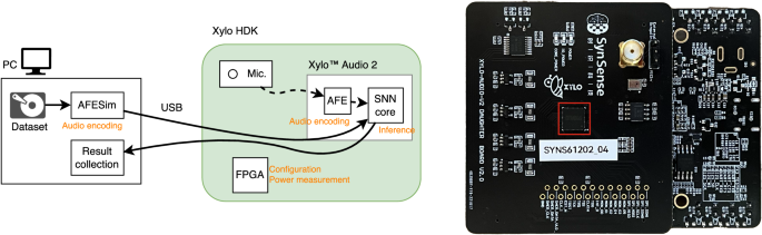
Left: Diagram of host and SUT communication. A simulator of the analog encoding module is run on a PC and streamed to the SNN inference core via USB. After inference, outputs are routed back to the PC for classification. An on-board FPGA configures and records power of the Xylo components. Right: The Xylo™ Audio 2 hardware development kit (HDK), used as the SUT. The red outline marks the Xylo inference module. Figures taken, with permission, from Ke et al.78.
Quadratic Unconstrained Binary Optimization (QUBO)
The processors ran repeatedly with five different initial variable assignments and seeds for different timeouts between 10−3 s and 103 s, and for different workloads sizes of up to 1000 variables. The neuromorphic algorithm is a parallelized version of simulated annealing that was running on a Kapoho Point board with one Loihi 2 chip, as shown in Fig. 10. The Loihi 2 board was controlled using Lava 0.8.0 and Lava Optimization 0.3.0. For comparison with conventional hardware, two solvers were adopted based on simulated annealing and tabu search, as implemented in the D-Wave Samplers v1.1.0 library80. The library was compiled on Ubuntu 20.04.6 LTS with GCC 9.4.0 and Python 3.8.10. CPU measurements were obtained on a machine with Intel Core i9-7920X CPU @ 2.90 GHz and 128GB of DDR4 RAM, using Intel SoC Watch for Linux OS 2023.2.0. All details on the solvers, benchmarking routine, and results have been provided by Pierro et al.57.
Fig. 10: A Kapoho Point board with Loihi 2 chips is connected to a host PC via ethernet.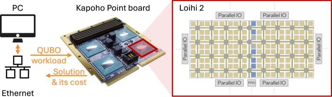
Shown here is a Kapoho Point board with 8 Loihi 2 chips, while the experiments were run on a board with 1 Loihi 2 chip. The QUBO workload is loaded onto the chip, and all processing happens on Loihi 2. On Loihi 2, the neuro-cores, in yellow, are arranged in two 8 × 8 grids and iteratively update the variables of the QUBO workload. Embedded CPUs, shown in blue, monitor the cost of the variable assignment. Six parallel IO ports enable 3D stacking of multiple chips for larger workloads than used here. An additional IO port provides the communication to the host PC. The energy and runtime measurements cover the computation of the Loihi 2 chip. Kapoho Point image courtesy of Intel.