
Specimen inclusion
The analyses are based on a dataset of 63 fossil specimens assigned to the genus Homo, complemented by data from recent modern humans. Inclusion of fossils in the analyses depended on their state of completeness for each of the anatomical regions analyzed (face and neurocranium). The neurocranium dataset included 57 specimens and the face included 47. Table S1 lists the fossils included in the final analyses with their contextual information (OTU assigned, chronological age, and percentage of missing values estimated). 24 complete skulls of modern Homo sapiens were added to the fossil specimens, to represent modern humans. The 24 individuals represent one male and one female randomly chosen from a larger sample of 233 individuals from 12 modern human populations worldwide, representing subsets of previously published samples22,23,24,25 (Table S1). This sample size was chosen to avoid the overrepresentation of modern humans in the calculation of the average covariance between landmarks.
Operational taxonomic units
To maximize the number of steps in the Homo evolutionary lineage in the tests of evolutionary scenarios, we classified the specimens into eight Operational Taxonomic Units (OTUs) along chronological and species boundaries (Table S6). In order to maximize specimens for each OTU we used the broadest definitions of these taxa (i.e., Homo erectus s.l., Homo heidelbergensis s.l., and early Homo)10. For Homo neanderthalensis and Homo sapiens, the chronological resolution available for the fossils and the larger sample sizes allowed them to be separated into more than one OTU to represent morphological trends over time. Table S6 presents the final breakdown of specimens per OTU for each of the datasets as well as their assumed chronological ranges. The OTUs represent different taxonomic levels, with some of them grouping fossils considered as being part of different species (early Homo includes H. rudolphensis and H. habilis) and other OTUs separating fossils of the same species into different chronological OTUs (early and late H. neaderthalensis, and early, Upper Paleolithic, and recent H. sapiens). This approach is consistent with the model-fitting methods adopted, as they do not require that similar taxonomic levels are represented, only that they are part of a lineage with relative chronology known for each of its steps. The models tested assume that the lineage was subject to the same evolutionary process across its entire existence, which means that the expected changes in trait values are proportional to the time that separates consecutive steps in the lineage. As such, OTUs chronologically close to each other are expected to show small changes compared to more distantly related steps. This proportional expectation of change is consistent with diachronic trends within a species as well as with changes between species. Parameters that are of larger relevance to the estimation of models’ goodness of fit are the mean and variance in each step and the number of steps in the lineage. Therefore, the lineages used in this study show a compromise between the bare minimum number of fossils in an OTU to allow a calculation of variance and the maximum number of OTUs that can be considered part of the lineage. However, the scarcity of the fossil record makes the statistical impact of our grouping decisions hard to evaluate. To address this limitation, we ran several alternative scenarios, with different combinations of OTUs or specimens in each OTU. All the analyses described in subsequent sections were replicated for the OTUs presented in Table S6 and for five alternative scenarios:
Alternative scenario A (Table S7) removed the two early Homo specimens, and started each lineage with H. erectus, to explore the impact of not having the earliest OTU, given that it is defined by only one specimen for each of two species (H. habilis and H. rudolphensis).
Alternative scenario B (Table S8) only includes the H. habilis specimen in the early Homo OTU, and assumes its measurements represent the average of the species. Variance of this OTU is defined as the average variance within all other OTUs.
Alternative scenario C (Table S9) only includes the H. rudolphensis specimen in the early Homo OTU, and assumes its measurements represent the average of the species. As with the previous scenario, variance of this OTU is defined as the average variance within all other OTUs.
Alternative Scenario D (Table S10) removed modern H. sapiens from the analyses, to make the results directly comparable to the results of the H. neanderthalensis lineage in terms of number of OTUs and approximate sample sizes.
Alternative scenario E (Table S11) joined all H. neanderthalensis fossils in a single OTU, to respect the currently accepted species boundaries for the species.
Morphometric data
Coordinate data were collected by KH using either a microscribe directly from specimens or digitally from 3D models. Landmarks were selected to represent overall craniofacial morphology, while minimizing missing information in the data (see below). The final datasets comprised 21 landmarks for the neurocranial and 23 landmarks for the facial datasets as subsets of previously published data22,23,24,25. Tables S2, S3 list the landmarks included in each dataset, as well as the percentage of missing data for each landmark.
Encephalization is best defined as the increase in cranial capacity relative to body size. As information on body size is not available for most specimens included in this study, we use changes in shape and changes in overall size as proxies to encephalization, given that encephalization in the genus Homo was accompanied by both significant changes in neurocranial architecture and in absolute size. Therefore, the shape analyses were conducted on a dataset scaled to size (see below) and our analysis of size was based on the calculation of the centroid size for each specimen. A similar approach was adopted for the analysis of facial reduction, as facial changes in the genus Homo are reflected in changes in shape and absolute size over the lineage.
Our neurocranial dataset is based on ectocranial landmarks (Table S2) and as such its variation is partially influenced by cranial osseous structures that are not directly related to brain size or shape. Nevertheless, we assume here that this variation is minimal and that the greatest component of the variance in neurocranial form is associated with brain size and shape, as the brain represents a large proportion of neurocranial volume in the genus Homo.
Estimation of missing data in the fossils was conducted in three steps. During data collection, when the morphological features allowed for accurate inference of landmarks missing, landmark coordinates were approximated. After data collection, bilateral landmarks were estimated by reflecting the side of available landmarks into the side of missing landmarks, following34. Finally, each dataset was trimmed to remove any specimen with more than 35% of landmarks missing. The trimmed datasets had their missing values estimated using thin-plate splines to interpolate landmarks missing34. The combination of these three steps of missing data estimation represents a necessary compromise to minimize the information missing in the original fossil record, while generating enough data points for the estimation of goodness-of-fit of the different evolutionary models. Although 35% is a high proportion of missing values, few fossils included have high percentage of missing values in the final dataset. The average percentages of missing values in the fossils for the neurocranial dataset is 3.82% and for the face it is 8.42% (See individual information in Table S1).
All individuals were transposed to the same origin, rotated to common axes of orientation, and scaled to the same size using Generalized Procrustes Analyses (GPA), and the transformed coordinates were used to calculate the Principal Components used in the tests of evolutionary models. Missing data estimation and GPA were performed in R35, using the geomorph package36,37.
Principal component analyses
The evolutionary models tested in this study are based on theoretical assumptions about changes of variance and means of linear traits over evolutionary lineages20, which require the 3D morphometric data to be converted into linear dimensions. In this study, we rotated the landmark coordinates through Principal Components Analysis and used the scores of the first four Principal Components as variables to be tested against the evolutionary models, as detailed below. The choice of using Principal Components Scores as measurements of morphological trends allows the morphometric information available in 3D data to be explored across the axes of largest variance in the dataset, without the need to explore combinations of linear measurements between landmarks. As the Principal Components with the largest eigenvalues represent the axes of largest shared variance of landmarks across the specimens in the dataset, they represent the most important dimensions of morphological change among Homo, and each of the OTUs can be visualized along those axes. Moreover, as the axes of largest shared variance in the data, they also correlate strongly with the dimensions of theoretical highest evolvability in Homo38,39, i.e., the dimensions along which more variance is available to be pulled by selective pressures in the environment. As such, the first Principal Components scores represent dimensions of morphological change with the highest potential for responding to selective pressures, and are in theory the most likely to show strong responses to selective evolutionary pressures.
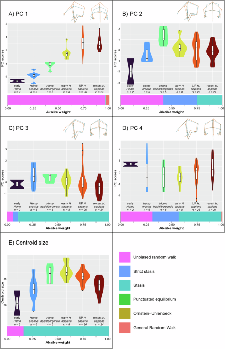
The evolutionary model fitting was limited to four Principal Components because the lower principal components explain smaller amounts of information, and are more influenced by variance within OTUs than variance that derives from differences between OTUs, which limits their explanatory power of morphological trends over time. In all datasets, the cumulative variance explained by the first four PCs is at least 50% of the variance in the original data. Details about the PCs’ eigenvalues and variance explained are reported in Table S4. The PC scores for specimens in each OTU were visualized through violin plots, and the morphological changes that are represented in each PC were illustrated by deforming wireframes connecting some of the landmarks to the minimum and maximum values observed in each PC. Principal components calculations and visualization were performed in R 4.5.235, supported by packages MASS40, ggplot241, and plotly42.
Analysis of size
The morphological analysis of shape variation represented through the Principal Component scores of the Procrustes-transformed data was complemented with the analysis of variation in size across the Homo lineage. Size changes were analyzed by extracting the centroid size of each specimen, calculated from the GPA analysis, and were analyzed via the model-testing procedure in the same way as the PC scores.
Evolutionary model testing
As defined by Hunt20,43,44, different evolutionary models can be conceptualized based on the magnitude and direction of trait averages’ change over time, in function of the variance observed in each of the lineage’s steps. As the expected outcomes of different evolutionary processes can be derived based on basic descriptive parameters of seriated samples (mean, variance, and relative time separating populations), they can be contrasted to observed data and their fit to the data can be quantified. Different evolutionary processes generate different expectations, and their relative goodness-of-fit to an evolutionary time series can be contrasted to other models using maximum likelihood estimates, which return the relative likelihood of different models tested to explain the variation and change observed in the measured data20.
Hunt43,44 derived the expectations of several distinct evolutionary models that can be fit against linear variables from seriated data. Here, we implement Hunt’s method to explore the evolutionary models that have the strongest fit to the craniofacial morphological variation of the genus Homo. We selected to test the fit of six different evolutionary models to the dimensions of morphological change defined by the Principal Components scores calculated from 3D morphometric data, as detailed before. The models tested are:
1.
General Random Walk (GRW): this model assumes that changes over time are the result of a biased walk, where changes in each step are drawn from a distribution with non-zero mean, and reflect the process that would be expected for lineages under a relatively constant and gradual directional selective pull from the environment. Under this model, evolutionary changes for each step in the lineage are drawn from a distribution with a non-zero mean step, which determines the direction of trait change, and variance that determines volatility of each step, which defines how much steps can vary from each other.
2.
Unbiased Random walk (URW): this model assumes that evolution is non-directional, and the accumulation of change over time is the product of the random sampling of the variance distribution at each step of the lineage. In this model, evolutionary changes at each step are drawn from a distribution with mean 0, and variance representing the volatility of each step. This model assumes that changes accumulate over time, but in a meandering way, representing stochastic or neutral evolutionary processes.
3.
Evolutionary Stasis (ES): this model assumes that there exists an optimum phenotype around which some variation is permitted, but due to the constraints acting to define the optimum, no accumulation of net morphological differences is seen over time. This model assumes that the traits for all steps are normally distributed around the optimal phenotype with a variance value that defines the magnitude of fluctuations that can be observed around the fixed mean.
4.
Strict Stasis (StS): This is a stricter version of the previous model, where all variation observed is assumed to be random noise and there is a strong pull around one same optimum phenotype across the entire lineage. The difference between this and the previous model is that in this stricter version of stasis, the expected variance around the optimal mean is zero.
5.
Ornstein-Uhlenbeck (OU): this model assumes that a population is orbiting around a nearby peak in the adaptive landscape, causing the trait to oscillate around the peak. The evolution towards the adaptive peak depends on the optimal trait value, and the strength of attraction to that optimal, variation of the distribution of which each step is taken (a measurement of genetic drift) and the value of the trait at the start of the evolutionary sequence.
6.
Punctuated Equilibrium (PE): this model assumes that there is a period of quick shift in the value of a trait, which separates periods of relative stability. Each period of stability in this case is defined by its own optimal value and variance around it. While the model accommodates the test of multiple possible steps of change, our analyses were limited to the search of only one step, due to the reduced number of OTUs available in our sequence. In this case, the model tests all possible steps in the evolutionary sequence where a shift could have occurred, reporting back the step that results in the strongest fit to the data.
The fit of different models can be compared to each other using maximum likelihood estimates and Akaike weights (standardized from the Akaike Information Criteria) are used to evaluate the relative plausibility of each model. The Akaike Information Criteria penalizes complex models over simpler ones, to avoid overfitting of models to the data and maximize the generalization that can be derived from the model. This is relevant to this study because in situations where the log likelihood between the different models is similar (i.e., that is, when there are no significant differences in how well models fit the data based on the maximum likelihood estimate), the Akaike weight will favor the simplest model. Model complexity is defined by the number of parameters included in each of the six models tested here. OU and PE are the more complex models (4 parameters), followed by GRW (3 parameters), then URW and ES (2 parameters) and finally StS (1 parameter). We use the Akaike weights in this study to contrast the fit of the different models to the Principal Components scores and to the centroid size of each dataset tested.
The evolutionary models tested assume that all steps in the temporal sequence tested are part of one single lineage, i.e., there is a direct ancestor-descendant relationship between all steps in the series. However, this is not a reasonable assumption in the genus Homo, especially when looking at the later taxa, given that Homo neanderthalensis and Homo sapiens are sister taxa, and the latter is not directly descended from the former. For this reason, we tested two different evolutionary sequences for Homo. The first one removes Homo neanderthalensis from the analysis, creating a time series that connects early Homo to archaic humans, to Homo sapiens (Table S1). The H. sapiens lineage is the most parsimonious sequence to explain the origin of modern humans through direct descent of the Homo fossils known to date. The second sequence removes all H. sapiens OTUs and, similar to the previous one, establishes a fossil sequence that leads directly to the appearance of Homo neanderthalensis. This H. neanderthalensis lineage explores the evolution of the Homo branch that led to H. neanderthalensis. However, it is a time series with a more limited number of OTUs and smaller sample sizes than the other lineage (Table S1). As described above, we explored five different alternative scenarios for these two lineages, changing the OTUs and fossils in them, to evaluate the biases introduced by our OTU definition, given the limited number of fossil specimens available to study.
For each lineage, we contrasted the fit of the six evolutionary models on two different datasets, to test our hypotheses. The first dataset considers only landmarks of the face and the second dataset only landmarks of the neurocranium. All model testing analyses were performed in R 4.5.2, using package PaleoTS45.
Analysis replicability
All analyses were conducted in R 4.5.2, using packages described in the previous sections. To permit the replication of the study, a commented document with all code, links to external resources, and results was compiled and is shared in html and quarto formats (Supplementary Code 1).
Reporting summary
Further information on research design is available in the Nature Portfolio Reporting Summary linked to this article.