
Why do coastal floods favor certain hours?
Coastal water levels are strongly shaped by tidal dynamics, particularly by the interaction between the principal lunar (M2) and solar (S2) tidal constituents. These constituents oscillate at slightly different frequencies, once per 12.42 h for M2 and once per 12.00 h for S2, producing a beat pattern that modulates the tidal amplitude, resulting in the spring-neap tidal cycle (Fig. 1a, b). The S2 phase lag sets the timing of spring tides, with the highest water levels occurring when M2 and S2 are in phase. Because the S2 constituent completes exactly two cycles per solar day, spring high water levels recur at two specific hours, namely those aligned with the S2 peaks.
Fig. 1: Tidal dynamics explain the intraday timing of flood peaks at Boston.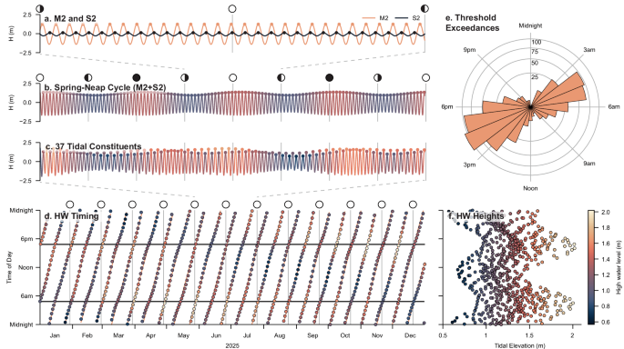
a heights of the principal lunar (M2, orange) and solar (S2, black) tidal constituents at Boston, MA (NOAA ID: 8443970) over half a lunar cycle; b combined M2 and S2 signal over two lunar cycles, illustrating spring-neap modulation; c full tidal prediction using all 37 NOAA tidal constituents (relative to NAVD88, the standard North American vertical datum); d timing (in UTC) and height of predicted tidal high waters in the year 2025 (relative to NAVD88); orange and black lines indicate the timing of M2 and S2 peaks, respectively; e timing of threshold exceedances above NOAA’s NOS minor flood level (2.078 m+NAVD88); f predicted tidal high water heights (relative to NAVD88) and their intraday timing. Colors in panels (b–d, f) indicate the height of local high water. Lunar phases are indicated in panels (a, b, d) by filled, open and half-filled circles, together with gray vertical grid lines.
Beyond the dominant M2 and S2 constituents, additional tidal components modulate the timing and amplitude of high waters (Fig. 1c, d). Diurnal constituents, primarily K1 and O1, generate once-daily oscillations that produce inequalities between successive high waters, which can cause the highest tides to occur preferentially at only one particular time of day. In predominantly diurnal regimes (Form factor > 3, see “methods”), this would yield no strong intraday clustering of peaks; however, interactions between K1 and smaller diurnal constituents such as P1 introduce amplitude modulations that still favor particular hours of the day.
On longer timescales, (semi-)annual constituents (Sa, Ssa) and phase locking between specific tidal pairs produce seasonal clustering of extreme tides33, such as S2-K2, S2-T2, K1-P1, or S2-K1. Semidiurnal tidal amplitudes typically peak around the equinoxes (March and September), whereas diurnal tides reach their maxima near the solstices (June and December). Non-tidal influences, including daily and seasonal variations in atmospheric pressure and wind patterns, may further enhance or shift this clustering34,35. At Boston, for instance, the annual highest tides typically occur in May and November, reflecting the combined seasonal modulation of diurnal and semidiurnal constituents (Fig. 1d). Supplementary Note 1 provides a mathematical framework for predicting when such phase-wrapping occurs, how many distinct peaks emerge in the solar reference frame, and over what interval the pattern repeats. This helps explain the emergence of intraday and intrayear clustering in tidal extremes.
The contribution of tidal dynamics to the timing of real-world flood events is exemplified using observational data from Boston, Massachusetts (Fig. 1e). Extreme high waters and threshold exceedance events show a marked concentration around specific hours of the day, consistent with patterns predicted by tidal constituent interactions. Notably, 70.4% of all exceedances above the NOAA National Ocean Service (NOS) minor high-tide flooding (HTF) threshold (hereafter the minor NOS threshold; 2.078 m + NAVD88 at Boston) occur within ±1.5 h of the dominant peak times. These peaks typically occur near 4 am and 4 pm UTC (corresponding to 11 pm and 11 am EST), forming a bimodal daily distribution. The slight skew toward the midday peak (43.2% of all exceedances) coincides with business hours and may amplify societal impacts. This preference for local noon and midnight has been noted historically25,26, and is consistent with the phase-locking behavior of key tidal constituents.
Spatial patterns in timing
Our analyses proceed from general high-water variability to events more directly associated with flooding. We first examine the timing of high water events with exceedance intervals of one year or less, as these provide a consistent and comparable basis across stations. We then assess whether these timing characteristics persist for subsets of events exceeding site-specific thresholds more directly linked to flooding.
The intraday timing of high water events with exceedance intervals of one year or less across coastal regions closely follows the spatial progression of the solar semidiurnal (S2) tidal wave (Fig. 2). To investigate the relevance of this spatial control, we classified each tidal station by its dominant exceedance timing (see “Methods”) and compared these classifications with the S2 phase distribution. Peak timing modes were identified by locating the three-hour window that contains the majority of threshold exceedances (Mode 1). After removing this block, a second three-hour window with the next highest concentration of exceedance peaks was identified as Mode 2. Prominence refers to the fraction of peaks that occur within each mode relative to the total. The sensitivity of peak hour and prominence to the chosen recurrence interval is explored in the Supplementary Fig. 1.
Fig. 2: Spatial patterns in the intra-day timing and prominence of threshold exceedance peaks across the US and UK.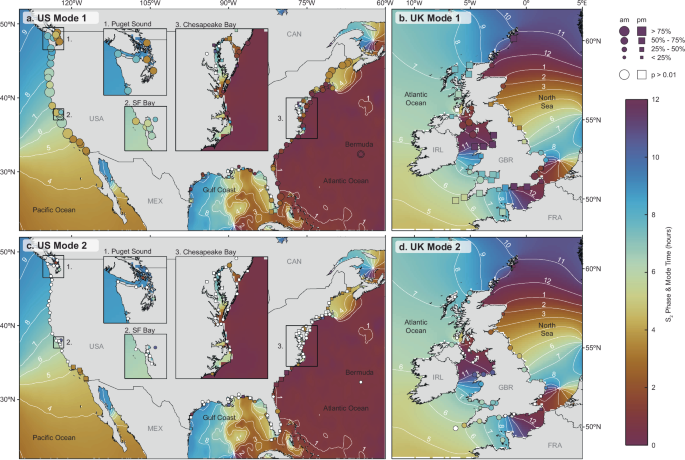
a, b First exceedance peak mode for the mainland US (a) and the UK (b), based on long-term tide gauge records. c, d Second mode for the same regions. Marker color indicates the time of day (in UTC), with round symbols denoting morning (AM) peaks and square symbols denoting afternoon (PM) peaks. Marker size reflects the prominence of the mode, defined as the percentage of annual exceedance events occurring within 1.5 h of the modal time. White-filled markers indicate locations where the distribution of peak times is not significantly different from a uniform distribution (p > 0.01). Inset maps in (a, c) highlight Puget Sound, San Francisco Bay, and Chesapeake Bay. The background shading shows the phase of the S2 tidal constituent relative to UTC, derived from the EOT20 global tidal model66. Coastlines and political boundaries from the Global Self-consistent, Hierarchical, High-resolution Geography database (GSHHG;67).
Along the West Coast of the US, the S2 tidal wave exhibits a clear northward progression, traveling from the Mexican to the Canadian border in approximately 5 hours. This results in a systematic shift in exceedance timing from south to north (Fig. 2a–c). This region displays some of the highest Mode 1 prominence values, particularly in the Pacific Northwest, reflecting a strong and temporally coherent daily peak. Mode 2 is generally not statistically significant, indicating a predominantly unimodal distribution (one prominent daily high water). In contrast, the southern US Pacific coast shows a higher prominence of Mode 2, suggesting a more bimodal pattern in exceedance timing.
On the US East Coast, peaks are more synchronized, and most locations experience threshold exceedances approximately at the same time. The prominence of Mode 1 is moderate (typically 25–50%), and Mode 2 is often not statistically significant, suggesting a more complex interaction between tidal and non-tidal influences. This widespread synchronization results from shelf co-oscillation, where tidal forcing reflects off the continental slope, producing a standing-wave pattern with a nearly uniform phase along the US East Coast coast36,37,38. A notable exception is the northern East Coast close to Canada, where local tidal dynamics in the Gulf of Maine introduce a 4–5 h delay in exceedance peak timing and enhance the prominence of both daily modes.
The Gulf Coast in the south of the US exhibits a more diffuse and less predictable pattern. Here, the tidal range is smaller (not shown), and the diurnal constituents dominate (Fig. 3a). Both the small tidal range and the dominance of the diurnal constituents result in weak clustering of the exceedance timing. Both Mode 1 and Mode 2 show low prominence, and the S2 wave progression is limited. This reduced regularity likely reflects the combined influence of diurnal tidal forcing and the frequent impact of tropical cyclones. These geographic contrasts mirror the regional division in which tides control HTF along the West Coast and in the Gulf of Maine, whereas non-tidal residuals dominate along most of the East Coast and the Gulf coast in the south39.
Fig. 3: Spatial patterns in the intra-year timing and prominence of threshold exceedance peaks across the US and UK.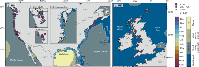
a, b First exceedance peak mode for the mainland US (a) and the UK (b), based on long-term tide gauge records. Marker color indicates the time of year of the dominant intra-year peak, while marker size reflects its prominence, defined as the percentage of annual exceedance events occurring within 1.5 months of the peak modal time. White-filled markers indicate locations where the distribution of peak dates is not significantly different from uniform (p > 0.01). The background shading shows the tidal form factor (F), calculated as (K1 + O1)/(M2 + S2), which reflects the relative influence of diurnal versus semidiurnal tidal constituents. Coastlines and political boundaries from the Global Self-consistent, Hierarchical, High-resolution Geography database (GSHHG;67).
In the UK, the exceedance timing closely follows the progression of the S2 tidal wave, although the presence of multiple amphidromic points introduces notable spatial complexity (Fig. 2b–d). Both Mode 1 and Mode 2 are prominent along much of the UK coastline, together indicating a high degree of temporal regularity. Most sites exhibit most exceedance peaks during the afternoon or evening hours (UTC), with a few exceptions in the southeast and southwest of the UK, where morning peaks are more common.
In semi-enclosed basins and estuaries, such as Puget Sound, Chesapeake Bay, and San Francisco Bay in the US, and the Bristol Channel in the UK, exceedance timing often lags behind that of the adjacent open coast. These lags reflect the inertial response of shallow water to the tide-generating forcing under the influence of local bathymetry and geometry and may amount to several hours (e.g., up to five hours at Philadelphia in the Delaware River). As a result, exceedance timing can vary substantially over short spatial scales, and mode prominence tends to be more spatially variable.
Across both the US and the UK, the first intra-year exceedance timing mode (Mode 1) exhibits strong temporal clustering, with slightly higher prominence observed at US tide gauge stations compared to the UK (Fig. 3). Along the West Coast of the US and the northern segment of the East Coast, peak timing is concentrated in December and January, reflecting enhanced diurnal tidal amplitudes around the winter solstice31. In contrast, the Gulf Coast and the Southeast US show peak timing between August and October. In the UK, peaks occur most frequently in January and February, although several sites exhibit earlier peaks in October and November. The timing of these annual peaks likely primarily reflects non-tidal influences, such as the regional storm season that dominates in the UK during winter months.
Balancing tides and storm surges
To assess the influence of tidal versus surges on exceedance timing, we use the ratio of the tidal range to the surge height corresponding to a once-per-year exceedance as a proxy for tidal dominance (see “Methods”). We find that regions with high tide-surge ratios, where tidal forcing dominates over non-tidal variability, exhibit stronger clustering and regularity in exceedance timing (Fig. 4a). For gauges with a ratio exceeding 2, the minimum prominence is 58.1%, with a median value of 89.0%.
Fig. 4: Influence of tidal dominance on the prominence of exceedance timing modes.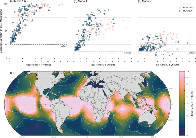
Subplot a shows the combined prominence of exceedance timing modes 1 and 2 (see “Methods” for details), expressed as the percentage of annual exceedance events occurring within ±1.5 h of the modal times. The prominence values are shown in relation to the tide-surge ratio, which is defined as the tidal range divided by the surge height corresponding to a once-per-year exceedance. Subplots b, c display the individual contributions of mode 1 and mode 2, respectively. Blue markers represent NOAA (US) tide gauge locations; pink markers represent BODC (UK) sites. Crosses indicate locations where the distribution of peak timings is not significantly different from a uniform distribution(p > 0.01). Dashed lines show expected values if peaks were evenly spread across the day (uniform distribution). Subplot d presents a global map of the tide-surge ratio, derived from the GTSM model40,41. The map was created by interpolating data from 43,119 GTSM output locations. High-latitude regions near the poles were excluded due to expected limitations in model performance. The underlying tidal range and 1-yr surge maps used to compute this ratio are provided in Supplementary Fig. 2. Coastlines and political boundaries in Subplot (d) are from the Global Self-consistent, Hierarchical, High-resolution Geography database (GSHHG;67).
The prominence of mode 1 is consistently elevated in these regions, indicating a robust primary timing signal. In contrast, the prominence of mode 2 varies depending on the diurnal inequality (difference between the two daily highs). Where tides exhibit high diurnal inequality, mode 1 tends to dominate, suppressing mode 2 prominence. This distinction is evident when comparing US and UK tide gauge sites. US locations, particularly along the west coast, generally show higher prominences in mode 1 and lower in mode 2 for similar tide-surge ratios, while UK sites often exhibit a substantial prominence in mode 2, approaching the theoretical maximum of 50%.
A global tide-surge ratio map, derived from predictions from the Global Tide and Surge Model (GTSM)40,41, extends these regional findings to a global context (Fig. 4). High ratios are observed near the equator, where storm surges are relatively low, and along the western coasts of the Americas and Euro-African continents. These regions are characterized by strong tidal dominance, and consequently, exceedance peak timing should be more predictable and temporally clustered. In contrast, areas with low ratios, such as those near amphidromic points or where surge variability is high, are expected to exhibit a weaker clustering of exceedance events. The observed spatial patterns are consistent with earlier results indicating strong clustering of exceedance timing in both the US West Coast and the UK. A limitation of this map is that it does not distinguish between tidal regimes. Diurnal tides show less clustering in the timing of daily peaks than semidiurnal tides, so intraday regularity is slightly reduced in diurnal or mixed regimes with comparable tidal ranges.
Timing patterns in observed coastal floods
Having established that tidal dynamics strongly govern the timing of water-level exceedances occurring once per year or less, we now examine how this regularity extends to actual flood events, those that cause measurable disruption or damage. We use standardized impact-based thresholds from the NOAA NOS42 for the US and the SurgeWatch database for the UK43 to distinguish between flood severities. NOS minor floods correspond to “nuisance” or “sunny-day” flooding, localized ponding or street flooding without major damage, while moderate floods cause road closures and structural damage. SurgeWatch moderate events (Category ≥ 3) meet at least three impact criteria, including inundated property, service disruption, extensive flood descriptors, or sea-defense damage. These consistent definitions allow us to assess whether tidal control extends to real, observed floods and to examine how their timing aligns with typical daily human activities (Fig. 5). We note that such thresholds provide a simplified representation of flood impacts; actual flooding can vary depending on local conditions, infrastructure, and processes (e.g., wave run-up, drainage, and flood pathways), and may not be fully captured by a single water-level threshold.
Fig. 5: Timing of flood events per station.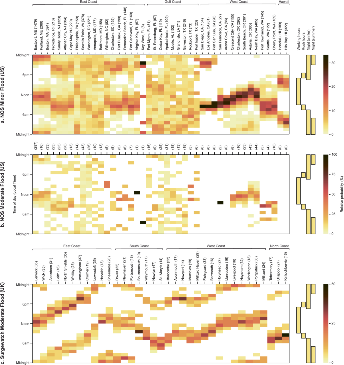
Hourly distribution of flood peaks exceeding impact-relevant thresholds at selected tide gauges along the US and UK coasts in local time. Sites were chosen to provide a representative spatial spread along both coastlines and to include well-known or metropolitan locations. a, b Relative probability of exceedances over NOAA NOS minor (a) and moderate (b) flood thresholds; c Timing of events classified as moderate or worse (Category 3 and higher) in the SurgeWatch database43. Probabilities are normalized per station to account for differing event counts (with the number in brackets specifying the number of floods per station). Time windows associated with varying societal vulnerability (e.g., working hours, rush hour, nighttime) are indicated by yellow bars next to each heatmap.
In the US, exceedances of the NOS minor flood threshold exhibit clear regional patterns (Fig. 5a). Along the Northeast Coast, the timing of floods is mostly clustered with bimodal peaks. From Eastport to Boston, these peaks are very pronounced and typically occur around noon and midnight local time, aligning with business hours and nighttime. South of Boston, the temporal organization remains evident, though slightly reduced. Flood peaks shift to the morning and evening, coinciding with morning commute periods, increasing the potential for transportation-related impacts. The Delaware (Cape May & Philadelphia) and Chesapeake Bay (Sewells Point to Baltimore) regions provide exceptions with weak clustering. Further south, parts of the Carolinas and Florida (Wilmington to Key West) retain moderate regularity, while the timing along the Gulf Coast remains largely unpredictable, shaped by small diurnal tides and frequent tropical cyclones.
The West Coast of the US displays some of the strongest temporal coherence. In Southern California (San Diego to Port San Luis), flood peaks align with the morning rush hour, while further north, timing shifts progressively later, aligning with midday business hours. Within Puget Sound (Port Townsend, Seattle & Cherry Point), flood peaks occur earlier than on the outer coast, again aligning with morning rush hour to early business hours. Hawai’i (Honolulu & Hilo Bay) also exhibits a bimodal pattern, with peaks in the early morning and late afternoon. At the moderate flood threshold (Fig. 5b), exceedances are less frequent, but predictable timing persists in several regions. The Northeast and Northwest Coasts continue to show clustering, albeit with reduced prominence.
In the UK, flood events classified as moderate or higher in the SurgeWatch database (Fig. 5c) show remarkable temporal regularity. Most locations exhibit bimodal peaks, with a clear spatial progression along the coast. Flood timing aligns with business hours, rush hours, or nighttime, depending on location. Notably, in the southeast UK (Harwich to Dover), where the 1953 North Sea flood caused significant loss of life, flood peaks occur in the middle of the night, a factor likely contributing to the high casualty rate15.