
Cohort selection and data sources
Our UCSF echocardiogram dataset comprised studies acquired on adult patients at UCSF between 2012 and 2020. These raw imaging data are linked with structured diagnoses and measurement data, including quantitative and qualitative measures adjudicated by level 3 echocardiographers at the UCSF echo lab. Measurement of RV parameters was standard practice in the UCSF echo lab during the study period; RV size and function labels were present for the majority of studies. Pixel data were extracted from the Digital Imaging and Communications in Medicine format, and the echo imaging region (cone) was identified by generating a mask of pixels with intensity changes over time. We then applied erosion and dilation operations to remove smaller moving elements such as electrocardiogram waveforms. Videos were then cropped to the smallest square that contained the entire echo imaging cone and resized to 224 × 224 pixels. All analyses excluded the following study types: transesophageal, intracardiac, and stress tests of any kind. This study was reviewed and received approval from the Institutional Review Boards of UCSF and the University of Montreal which waived the need to obtain informed consent in the setting of this minimal-risk retrospective record research.
To train the video-based view classifier, 6,549 echocardiograms from 1,437 patients were manually labeled. The 20 most common views were labeled, with the remainder classified as “other.” To simulate real-world data flow where all clinically obtained videos would undergo view classification, “other” was included as a trained class for the DNN. Views in the “other” class included view from transesophageal echo, color compare, split screen, among others. By training the DNN view classifier to classify 21 distinct echo views, more views than previously published image-based view classifiers, this served to reduce input variance into the DNN; this allows for discrimination, for example, between standard depth PLAX views, PLAX zoomed on the left atrium, or PLAX zoomed on the aortic valve16. This view classifier DNN achieved a mean AUC of 0.972 across the 21 classes (Extended Data Fig. 1). We trained a similar video-based DNN to classify the presence or absence of color doppler within the echo video which achieved an AUC of 0.991 (Extended Data Fig. 1).
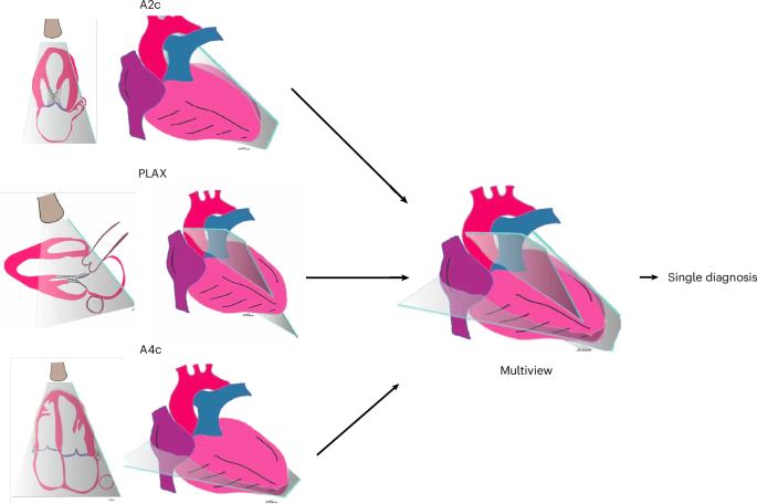
These view/doppler-classifier DNNs automatically identified input echo videos comprising the predefined view and doppler combination for each task. We then applied these view/doppler DNN classifiers to all UCSF echos to identify the specific echo videos needed for training and validation for each of the three demonstration tasks. For the ventricular abnormality and diastolic dysfunction multiview DNNs, the three input echo views used were non-doppler A4c, A2c, and PLAX views; and for valve regurgitation, the input echo views were color-doppler A4c, A5c, and PLAX views. To ensure a fair comparison between single-view and multiview models, we first excluded all studies that were missing any required views. Both model types were trained and evaluated on videos from the same studies, the only difference being whether a model received a single view or three views as input.
For the ventricular abnormality dataset, we included all patients in our dataset with measures of ventricular function, comprising 36,023 echo studies from 11,334 patients. Of these, 2,907 patients were identified as having a ventricular abnormality, defined as having any abnormal measure of EF, LV size, RV size, or RV function. Ventricular abnormality was defined as positive if there was any abnormality in LV/RV size or function. LV size abnormality was defined as greater than mild dilation, which was LV end diastolic volume index of >86 ml m−2 for men or >70 ml m−2 for women. LV functional abnormality was defined as LVEF < 50%, measured by Simpson’s biplane approach19. RV size abnormality was defined as moderately increased or greater, and abnormal RV function was defined as moderately decreased or greater19.
For diastolic dysfunction, we included all patients with measures of diastolic dysfunction, comprising 11,341 echo studies from 6,649 patients. Diastolic dysfunction was defined as any diastolic dysfunction (grades 1–4) as determined by ASE guidelines20,21. Of these, we identified 4,774 patients showing any diastolic dysfunction measure above grade 0. Grades 1–2 included any annotation of abnormal or impaired relaxation, or increased filling pressure. Grade 3 included all pseudonormal diastolic function, and grade 4 included restrictive diastolic function.
For valve regurgitation, we included all patients with measures of valve regurgitation, comprising 27,652 echo studies from 18,533 patients. Any substantial valve regurgitation was defined as moderate or greater regurgitation in any of the mitral, tricuspid, or aortic valves according to ASE guidelines22. Of these, we identified 969 patients with mitral valve regurgitation, 329 patients with aortic valve regurgitation, and 1,299 patients with tricuspid valve regurgitation.
Our external validation dataset consisted of all echos acquired at the MHI in 2022 on patients over the age of 18 years. These studies were similarly linked to the clinical echo reports from which we obtained qualitative and quantitative reference labels. The MHI echo lab uses linear measurements (compared with volumetric measurements at UCSF), which resulted in our needing to use linear measurements to define certain “abnormal” findings at MHI, as described below. For LV function, we labelled studies with an EF < 50% to be abnormal. Studies with a basal RV size measurement >4.4 cm were labelled abnormal. Studies with a basal LV size measurement of 6.3 cm for men or 5.6 cm for women were defined to be abnormal. For RV function, abnormality was defined as more than moderately decreased function (qualitative). Diastolic function grade labels were available in MHI and followed ASE guidelines20,21. Measurement of RV parameters was standard practice in the MHI echo lab during the study period. MHI echos were processed using identical preprocessing as described above. Preprocessing and view classification performance in MHI were assessed by randomly reviewing 350 MHI clips labelled by the UCSF-trained view classifier. The view classifier performed well across our target views with precision (PPV) of 100% for A4c, 83.3% for PLAX, 88.5% for A2c, and 81.8% for A5c, with a global accuracy of 79.14%. We deployed our trained multiview DNNs on all MHI echos that had pertinent diagnostic labels and the three predefined views for each task. We then ran inference using the three multiview DNNs on all MHI studies containing the appropriate views.
DNN architectures
For view classification, doppler detection, and all single-view models, we chose as our video-based DNN backbone the 3D convolutional neural network X3D-Medium (X3D-M), from the family of X3D architectures15. We tested other video-based DNN backbones, including R2-1D and the transformers ViViT, MoviNet, and STAM, and found X3D the most performant backbone overall. X3D-M had the additional benefit of being relatively lightweight compared to these other models, with 3.8 million parameters compared to R2-1D’s 33.3 million. This computational efficiency enabled faster training, larger batch sizes, and, eventually, expansion of the architecture to incorporate multiview video input.
For our multiview analysis, we developed a bespoke architecture to integrate multiple views with an enhanced mid-fusion strategy. First, the DNN passes each view, consisting of a 64 × 224 × 224 × 3 video, through five convolutional blocks consisting of 3D convolutions, batch normalization, and a rectified linear unit non-linearity, producing temporally and spatially reduced embeddings of shape (B, C, T, H, W) representing batch, channel, time, height, and width. These first five blocks are unchanged from the original X3D-M architecture15. The resulting embeddings are stacked along a new view dimension, V, to produce a tensor of shape (B, C, V, T, H, W). This tensor is then flattened across the time, height, and width dimensions, resulting in a tensor of shape (B, C, V, THW). A sixth convolutional block (following the same convolution, batch normalization, rectified linear unit format) performs a 2D convolution across the view and combined spatiotemporal dimensions to fuse information across the views. The tensor is then reshaped to (B, CT, V, H, W) and passed to the final convolutional block. This final block expands the number of channels by a factor of 128 as it performs a 3D convolution across view, height, and width. This step is crucial for deep integration of spatiotemporal information across views. The resulting tensor is then reshaped to (B, CV, T, H, W), and we perform average pooling on time, height and width dimensions before passing the final tensor through a fully connected layer and a decision head. The final multiview DNN has 230 million parameters.
DNN training
All DNNs were developed and trained in Python (version 3.8.8) using the Pytorch library35 (version 1.8.8). Training of single-view DNNs took approximately 3 h; training of multiview DNNs took approximately 30–50 h on dual NVIDIA Quadro RTX 8000. For binary classification, we used a sigmoid decision head and the binary cross entropy loss, and for multiclass classification, we used a softmax decision head and the cross entropy loss function. For each of the three demonstration echo tasks separately, the data were divided into training/development/test datasets specific to that task in a 70/15/15 ratio, split by patient. The development dataset was used during training for learning rate decay scheduling and selection of the final models. The test dataset was held out from any model training or development and used to calculate evaluation metrics once the final DNNs for each task were trained.
Input videos to the DNN consisted of the first 64 frames of the video. Videos shorter than 64 frames were padded with empty frames. Echo video frame rates were 33 ± 17 frames per second. We did not normalize frame rates in the final training process, as this was tried and did not improve performance. The view classifier DNN was trained for 1,000 epochs starting with a learning rate of 0.01 and reducing learning rate using a factor of 0.5 with a patience of 50 and a loss threshold of 0.01. A separate doppler detection algorithm was trained on the same data with the same parameters. After training, the checkpoint achieving the lowest loss on the validation set was selected as the final DNN.
To train the single- and multiview DNNs, we used a standard hyperparameter sweep paradigm to allow all models to achieve their optimal performance and enable comparison. We performed separate hyperparameter sweeps over identical ranges of learning rate, threshold, and patience for learning rate decay for each task and view combination. For each sweep, we sampled learning rate from a log-uniform distribution between 1 × 10⁻⁶ and 5 × 10⁻². For learning rate decay, we used the ReduceLRonPlateau scheduler monitoring validation loss with a 5% threshold. The scheduler patience was randomly sampled from (3, 5, 7, 10) and factor from (0.3, 0.5, 0.7). All models were trained for a total of 50 epochs without early stopping over 40 sweep trials with fixed random seeds for reproducibility. All models were trained on a single fixed data split for each task dataset. Both the input data size and model parameter sizes are substantially larger for the multiview DNNs resulting in increased training time for multiview models. We used the stochastic gradient descent optimizer (momentum = 0.9; weight decay = 0.0001) for all training runs. Training data were augmented gently using random resized crop between 0.95 and 1.0, color jitter between 0.8 and 1.2, and random rotation between −5 and 5 degrees. After training, the checkpoint achieving the highest AUC on the development set was selected as the final DNN.
All DNNs were evaluated using a combination of AUC and sensitivity/specificity at an optimal threshold defined as the threshold at which the geometric mean of sensitivity and specificity was maximal. Multiclass DNNs were evaluated using the mean AUC per class.
Explainability analysis
To examine the features from the input video that contributed to the DNN predictions, we used a custom adaptation of the guided class-discriminative gradient class activation mapping algorithm (guided grad-CAM) to examine single-view model performance23. This adapted the 2D implementation to expand the dimensionality to accommodate 3D video data. This provides an approximation of what echo video pixels the multiview DNN model may be focusing on, with the caveat that these are single-view approximations. Representative videos were chosen for high diagnostic quality and confident disease-positive predictions (>0.95), and the adapted guided grad-CAM approach was used to generate heat maps corresponding to the pixels that most strongly contributed to that DNN’s prediction. In addition to the guided grad-CAM, we also generated standard grad-CAM maps to provide a course, class-discriminative localization of relevant regions, while guided grad-CAM highlights fine-grained pixel-level features.
Statistical analysis
All continuous values are presented as mean ± 95% CI. For binary classification DNNs, the output of the final sigmoid function was a score ranging [0–1]. We report performance metrics using a default threshold for each DNN that was selected to maximize the F1 score on the development dataset for each task36. For the sensitivity/specificity-optimized sensitivity analysis, DNN performance metrics are reported at thresholds in the test dataset that fix sensitivity or specificity at 0.800. Statistical analyses were conducted in Python using pandas 2.3.0, numpy 1.26.4, scikit-learn 1.6.1, statsmodels 0.14.5, and MLstatkit 0.1.7.
The multiclass view classification DNN output consists of 21 continuous values ranging [0–1] with the predicted view corresponding to the maximum of the 21 values. For all test datasets, we present the AUC, sensitivity, specificity, and F1 score. CIs were derived by sampling the test set with replacement for 1,000 iterations to obtain 5th and 95th percentile values.
Differences in AUCs were tested using DeLong’s test37; in settings of multiple comparisons, Bonferroni correction was performed by adjusting the P values while retaining the threshold for significance at <0.05 (ref. 38). DeLong’s test was implemented using the MLstatkit package (version 0.1.7) in Python, and Bonferroni correction was implemented using the statsmodels package (version 0.14.5) in Python. Statistical significance was defined as P < 0.05.
For stratified analyses, we computed performance metrics for each DNN separately on strata of the test sets regarding age, gender, and disease subtypes. We defined disease substrata as those studies meeting previously described criteria for each abnormality compared to studies without criteria for abnormalities within each of the three echo tasks separately.
Reporting summary
Further information on research design is available in the Nature Portfolio Reporting Summary linked to this article.