
Climate scenarios and construction
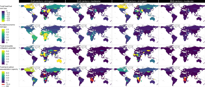
In this study, we selected SSP2 as a representative middle-of-the-road socioeconomic pathway to examine the spatial and temporal patterns of global climate-mitigation-related assets. SSP2 reflects intermediate assumptions regarding demographic change, economic development and technological progress, and is widely used as a reference scenario in climate impact and mitigation studies51. To isolate the effects of mitigation intensity while maintaining consistent socioeconomic assumptions, we examined three SSP2-based pathways spanning a range of climate-policy ambition levels. SSP2-2.6 represents a relatively stringent mitigation pathway; SSP2-4.5 represents a moderate mitigation pathway; SSP2-6.0 serves as the baseline scenario, representing a higher-emissions pathway with comparatively limited mitigation efforts, consistent with its characterization in the SSP database52. This scenario framework attributes differences across pathways primarily to mitigation ambition rather than to broader socioeconomic transformations. We assessed each indicator over two periods: mid-century (2020–2050) and end-century (2020–2100).
For the simulation of energy and economic conditions from 2020 to 2100, we utilized data from the AR6 database (Supplementary Table 2). Land-use and land-cover data were derived from the land-use components of three IAMs: REMIND–MAgPIE27,34, GCAM–Demeter35 and IMAGE36. These models provide comprehensive projections of land-use dynamics under different socioeconomic and climate scenarios. Additionally, climate variables were obtained from six general circulation models within CMIP653 (Supplementary Table 3). Both land-use data and climate variables were used to estimate renewable energy potential, while climate variables were also incorporated into economic damage projections. All spatial datasets were harmonized to a common spatial resolution of 0.5° × 0.5°. To reduce potential biases associated with coarse-resolution gridded data, we excluded countries with land areas below 2,500 km2 from the analysis.
Fossil fuel rent loss
The fossil fuel rent losses were calculated using data obtained from IAMs in the AR6 database. The data were extracted by filtering for SSP2 scenarios and global median forcing values (Supplementary Fig. 4). First, the regional revenue of each fossil fuel type (coal, oil and gas) was estimated based on production and price data for each model.
To allocate regional fossil fuel production from IAM scenarios to individual countries, we constructed a time-varying weighting scheme that combines information on current production and proved reserves. In the base year, country shares reflect observed production patterns, capturing existing extraction infrastructure, investment and institutional conditions. Over time, the allocation gradually incorporates information on proved reserves, reflecting their increasing relevance for long-term fossil fuel supply potential. Country-level production for fuel type f in country i and year t is given by
$${\mathrm{Prod}}_{i,t}^{f}={\mathrm{Prod}}_{r,t}^{f}\times\left[\left(1-{\lambda }_{t}\right){\mathrm{Share}}_{i}^{\mathrm{prod},f}+{{\lambda }_{t}\mathrm{Share}}_{i}^{\mathrm{res},f}\right]$$
(1)
where \({\mathrm{Prod}}_{r,t}^{f}\) is total production in region r from IAM scenarios, \({\mathrm{Share}}_{i}^{\mathrm{prod},f}\) is the country’s share of regional production in the base year and \({\mathrm{Share}}_{i}^{\mathrm{res},f}\) is the country’s share of regional proved reserves in the base year. The parameter \({\lambda }_{t}\in [\mathrm{0,1}]\) determines the relative contribution of reserves, and increases over time. It reflects a gradual shift from production-driven allocation in the short term to a greater role of reserve endowment in the long term. In the main text, \({\lambda }_{t}\) increases linearly from 0 in 2020 to 0.6 in 2100.
Country-level fossil fuel production and reserve data were compiled from multiple data sources as described in Supplementary Information, section 1. The value of each fossil fuel type was discounted and summed over mid-century (2020–2050) and end-century (2020–2100), and then divided by cumulative discounted GDP to express the country-level fossil fuel rent for each scenario. Rent losses were determined as the difference between SSP2-2.6 and SSP2-6.0 for the stringent scenario, and between SSP2-4.5 and SSP2-6.0 for the moderate scenario. Country-level GDP was sourced from the SSP database54. We employed a primary discount rate of 3%, with additional sensitivity analyses using 2%, 4% and 5% discount rates to capture the impact of different discounting assumptions on the results (Supplementary Fig. 5.1).
Robustness to alternative parameterizations of \({\lambda }_{t}\), including different terminal values and functional forms, is assessed in Supplementary Information, section 1. In addition, we conducted stress tests using extreme reserve-dependence pathways in which \({\lambda }_{t}\) reaches 1 by 2050, 2075 or 2100. Under these specifications, country-level allocation becomes fully reserve-based after the corresponding year. These scenarios are not intended as central assumptions, but rather as upper-bound tests of the influence of reserve dependence on country-level fossil fuel rent-loss estimates. Although this allocation framework allows country-level production shares to evolve over time through increasing reserve weighting, it does not explicitly capture future changes arising from extraction costs, reserve depletion, geopolitical disruptions, trade restructuring or evolving energy security strategies. Owing to the lack of globally consistent long-term data describing these processes, proved reserves are used as a practical proxy for long-term supply potential. Because proved reserves depend on current economic and technological conditions, they should not be interpreted as representing the full geological resource base.
Economic damage
Using CMIP6 datasets, we calculated the population-weighted annual temperature at the country level for the historical period (1985–2014) and for three future scenarios. We assessed economic impacts at the country level using both growth-based and level-based damage functions, following previous studies1,13,30. These damage functions estimate the impacts of temperature change on GDP and thereby represent aggregate macroeconomic climate damages. For growth-based functions, we applied the BHM and DJO models. GDP per capita was calculated using equation (2):
$${\mathrm{GDP}}_{r,t}={\mathrm{GDP}}_{r,t-1}\times\left(1+{\eta }_{r,t}+\delta \left({T}_{r,t}\right)\right)$$
(2)
where \({\eta }_{r,t}\) is the growth rate projected under SSP reference pathways (assuming no climate change) and \(\delta ({T}_{r,t})\) is a function of temperature change for country r in year t. For the BHM model, we used 1,000 bootstrap parameter sets derived from ref. 1 to measure the uncertainty in the temperature–growth relationship. The BHM models include both short-run (0-lag) and long-run (5-lag) specifications to measure immediate and delayed economic responses to temperature increases, while the DJO model applies cumulative 5-lag temperature effects to annual temperature changes in GDP growth rates9,30.
For the level-based damage functions, we estimated country-level economic impacts as output losses relative to a no-climate-change (‘non-cc’) scenario and can be represented as
$${\mathrm{GDP}}\ {\mathrm{loss}}_{r,t}={\mathrm{GDP}}^{\mathrm{non-cc}}_{r,t}\times D(T_{r,t})$$
(3)
where \(D({T}_{r,t})\) is a damage function representing the percentage loss in GDP due to climate impacts at temperature \({T}_{r,t}\). \({\mathrm{GDP}}_{r,t}^{\mathrm{non}\text-\mathrm{cc}}\) is the reference GDP from the SSP2 socioeconomic pathway for country r in year t. We used the Kalkuhl–Wenz subnational function, Tol’s meta-analysis function and Hope’s linear damage function to estimate economic impact, following the parameterizations outlined in prior studies31,32,33,55,56. All model parameters and specifications are provided in Supplementary Information, section 2 and the accompanying coding materials for reproducibility.
We then calculated avoided damages as the difference in cumulative discounted damages between the mitigation scenarios and the baseline scenario. To facilitate cross-country comparability and consistency with the other mitigation-related dimensions in our analysis, the avoided cumulative discounted damages were expressed as a share of cumulative discounted GDP. Similar to the evaluation of fossil fuel rent losses, we applied the same range of discount rates to calculate the avoided economic damages by mid- and end-century (Supplementary Fig. 5.2). Final estimates were derived using a two-step function median, first summarizing matched climate-model estimates within each damage-function specification and then taking the median across damage functions. Sensitivity analysis shows that growth-based damage functions yield higher median estimates and greater cross-country dispersion than level-based functions, while the final function-median estimate remains between the two groups (Supplementary Information, section 2.4).
Mitigation potential of renewable energy
The technical potential for renewable energy generation from PV and wind power is estimated using climate and land suitability factors. Climatic variables were sourced from the CMIP6 datasets, while land-use data were obtained from REMIND–MAgPIE, GCAM–Demeter and IMAGE. The potential power generation from utility PV systems in each grid i and year t (Eupvi,t) is calculated using equation (4):
$${\mathrm{Eupv}}_{i,t}={I}_{i,t}\times {h}\times {\mathrm{LSF}}_{i,t}\times {\mathrm{Area}}_{i,t}\times {\eta }_{\mathrm{PV},i,t}\times {\eta }_{\mathrm{LPV}}\times {P}_{R}$$
(4)
where \({I}_{i}\) is the solar irradiance (kw m−2, daily average in a year) in grid i (0.5° × 0.5°) in year t; h is the number of hours in a year (8,760); \({\mathrm{LSF}}_{i,t}\times {\mathrm{Area}}_{i,t}\) is the suitable land area in grid i in year t, which depends on the land suitability factor (LSF)57 and land-cover types; \({\eta }_{\mathrm{PV},i,t}\) is the panel efficiency, which is corrected by the atmospheric variables58 (the calculation method is listed in Supplementary Information, section 3.1); \({\eta }_{\mathrm{LPV}}\) is the land-use packing factor (0.47)7; and \({P}_{R}\) is the performance ratio between the actual power output and the standard test conditions due to losses such as transmission, cable and inverter losses (85%)7.
To project the potential power generation from rooftop PV in each grid i and year t (Erpvi,t), we incorporated regional variations and building characteristics using equation (5):
$${\mathrm{Erpv}}_{i,t}={I}_{i,t}\times {h}\times {\mathrm{FA}}_{r,t}\times {\mathrm{Pop}}_{i,t}\times {\beta }_{r}\times s\times {\eta }_{\mathrm{PV},i,t}\times {P}_{R}$$
(5)
where \({\mathrm{FA}}_{r,t}\) is the building floor area per capita, differentiated by rural and urban residents in region r; \({\mathrm{Pop}}_{i,t}\) is the population (persons), also separated by rural and urban residents in grid i; \({\beta }_{r}\) is the region-specific coefficient for converting floor area to roof area (Supplementary Fig. 6); and s is the architecturally suitability factor of the rooftop (0.32; ref. 7). Gridded rural and urban population data are sourced from Jones and O’Neill’s research59.
The potential wind power generation for each grid cell i and year t (Ewi,t) is calculated using equation (6):
$${\mathrm{Ew}}_{i,t}={{\mathrm{WPD}}_{\max }\times \mathrm{CF}}_{i,t}\times {h}\times {\mathrm{LSF}}_{i,t}\times {\mathrm{Area}}_{i,t}\times {\eta }_{1\mathrm{wind}}\times {\eta }_{2\mathrm{wind}}$$
(6)
where \({\mathrm{WPD}}_{\max }\) is the maximum wind power density (4 MW km−2) and \({\mathrm{CF}}_{i,t}\) is the ratio of predicted actual energy output to the maximum output in grid i (0.5° × 0.5°) in year t. The detailed calculation methods of \({\mathrm{CF}}_{i,t}\) are provided in Supplementary Information, section 3.2. \({\mathrm{LSF}}_{i,t}\) denotes the land suitability factor relevant to land-use types (Supplementary Table 4), and \({\mathrm{LSF}}_{i,t}\times {\mathrm{Area}}_{i,t}\) is the suitable land (onshore)/sea area (offshore) in grid i in year t. For the onshore wind power potential, three land-use datasets are utilized to estimate land suitability factors57. \({\eta }_{1\mathrm{wind}}\) is the annual availability of a wind turbine due to maintenance (95%)7 and \({\eta }_{2\mathrm{wind}}\) is the wind farm array efficiency (90%)7.
The technical potential of renewable energy (‘Potential RE’) type k in country c, \(\mathrm{Potential}\,{\mathrm{RE}}_{c,k,t}\), is the sum of—separately—\({\mathrm{Eupv}}_{i,t}\), \({\mathrm{Erpv}}_{i,t}\) and \({{Ew}}_{i,t}\) over the grid cells occupied by each country.
To give an economic value of the natural resources for energy generation of each renewable energy type needed for climate change mitigation, we scale each country’s technical potential with the share of total regional potential generation that is utilized for electricity generated through renewables in the mitigation scenarios compared to the baseline with data from the AR6 (Supplementary Fig. 2). To monetize the scaled technical potential, we multiply the scaled technical potential with the carbon intensity of electricity generation in the baseline scenario to give the potential to avoid emissions in each country using their renewable energy resources (data from AR6). Finally, we multiply the potential to avoid emissions with the carbon price in the mitigation scenarios (data from AR6):
$$\begin{array}{l}{\mathrm{MP}}_{c,k,t}^{m}={\mathrm{CP}}_{R,k,t}^{m}\times {\mathrm{CI}}_{R,t}^{b}\times \frac{\left({{\mathrm{Generated}}\,{\mathrm{RE}}}_{R,k,t}^{m}-{{\mathrm{Generated}}\,{\mathrm{RE}}}_{R,k,t}^{b}\right)}{{{\mathrm{Potential}}\,{\mathrm{RE}}}_{R,k,t}}\\ \qquad\quad\;\times \mathrm{Potential}\,{\mathrm{RE}}_{c,k,t}\end{array}$$
(7)
where \({\mathrm{CI}}_{R,t}^{b}\) is the carbon intensity of electricity generation in the baseline scenario, and \({\mathrm{Generated}\,\mathrm{RE}}_{R,k,t}^{m}\) and \({\mathrm{Generated}\,\mathrm{RE}}_{R,k,t}^{b}\) are the renewable electricity generation under the mitigation and baseline scenarios, respectively. \({\mathrm{CP}}_{R,t}^{m}\) is the carbon price under the mitigation scenario, \({\mathrm{MP}}_{c,k,t}^{m}\) represents the monetized mitigation potential for each country c, and \(\mathrm{Potential}\,{\mathrm{RE}}_{R,k,t}\) is the total technical potential in the region the country belongs to.
Finally, the discounted cumulative mitigation potential is divided by the discounted cumulative GDP for mid-century and end-century assessments across different discount rates (Supplementary Fig. 5.3).
Land carbon stocks and sequestration capacity
To assess land carbon sequestration capacity, we monetized it by multiplying annual carbon sequestration with the corresponding carbon price. Carbon prices are sourced from AR6, where countries within the same region share a common value. Annual carbon sequestration is calculated as the difference in land carbon stocks between consecutive years (\(\mathrm{Carbon}\,{\mathrm{stock}}_{t}-\mathrm{Carbon}\,{\mathrm{stock}}_{t-1}\)). The data are disaggregated at a 0.5° resolution using MAgPIE–LPJmL model outputs60 and subsequently re-aggregated to the country level.
Land-use projections are generated by MAgPIE, while LPJmL provides biophysical constraints on land productivity, water availability and carbon stocks. In the two mitigation scenarios, MAgPIE simulates active land-based mitigation in response to carbon prices, bioenergy demand and land-use targets. The moderate and stringent mitigation scenarios apply land-use targets from nationally determined contributions for afforestation, deforestation and land conversion. They differ in their GHG-price and second-generation bioenergy-demand pathways, which are aligned with cumulative emission budgets of 1,000 GtCO2 and 650 GtCO2, respectively. Mitigation uptake is constrained by competing demands for land from food, feed, seed and timber production, as well as by protected areas, conversion emissions, opportunity costs and temporal lags in carbon-stock development60.
This approach accounts for sequestration potential across various land types, including primary forests, secondary forests, pasture, cropland and managed forestry. We categorize primary and secondary forests as natural carbon sequestration resources, while pasture, cropland and managed forestry are considered human-managed sequestration resources. Similarly, the discounted cumulative value of carbon sequestration capacity under two mitigation scenarios is divided by the discounted cumulative GDP for mid-century and end-century assessments across different discount rates (Supplementary Fig. 5.4).
Cluster and similarity analysis
To ensure comparability across different indicators while preserving variance among mitigation scenarios and time periods, asset indicator values are capped at the 2.5th and 97.5th percentiles to reduce the influence of extreme outliers and normalized within each key variable using \(\frac{x}{\max (\left|x\right|)}\) before clustering. This approach maintains the relative magnitudes of values across all periods (mid- and end-century) and mitigation scenarios (moderate and stringent) while ensuring that positive and negative signs are retained to reflect directional impacts. The k-means clustering analysis is conducted using broad indicators to identify distinct country groups based on their overall economic and environmental stakes in climate mitigation. The four key clustering variables are total fossil fuel rent loss, avoided economic damage, total renewable mitigation potential and total carbon sequestration capacity.
Following the clustering analysis, a Euclidean-distance-based similarity analysis is applied to examine cross-country similarities in indicator profiles at a more detailed level. The similarity coefficient between countries i and j is defined as
$${\mathrm{Similarity}}_{{ij}}=\frac{1}{1+\sqrt{{\sum }_{k=1}^{n}{\left({x}_{{ik}}-{x}_{{jk}}\right)}^{2}}}$$
(8)
where \({x}_{{ik}}\) and \({x}_{{jk}}\) are the normalized values of indicator k for countries i and j, respectively, and n is the total number of indicators. The coefficient ranges between 0 and 1, where 1 indicates identical profiles and values closer to 0 indicate greater dissimilarity.
This analysis focuses on sub-dimensional indicators to assess how countries compare in terms of their specific resource and economic characteristics. The key metrics used for similarity analysis include fossil fuel rent loss (coal, oil, gas), renewable energy potential (solar, wind), avoided economic damage, natural carbon sequestration capacity and managed carbon sequestration capacity.