
Design of nonreciprocal cells and network strategy
The 8-input 8-output nonreciprocal network consists of 4 reciprocal cells and 3 nonreciprocal cells, as shown in Fig. 2a. With well-matched mode impedances, the ports of these computational cells can serve as the basic low-reflection nodes in the multi-port network. Through layer-by-layer cascading of nodes, we construct an integrated computing network capable of reconfigurable multi-channel transmission. It is worth noting that we use staggered interconnected cells to cascade four layers of nodes. This approach enhances coupling between cells, allowing flexible adjustment of nonreciprocal transmission of the overall network. In this interleaved, interconnected structure, there are not only cross-connections and direct connections between nodes across layers, but also interconnections among nodes within each layer. Notably, the nodes exhibit four distinct connection modes: reciprocal (R), nonreciprocal (NR), FP, and BP connections. R and NR connections work simultaneously in bidirectional pathways. In contrast, FP or BP connection operates through a single pathway. In other words, FP and BP connections can only be “activated” by signals reflected from the (i + 1)th layer back to the ith layer. Therefore, the interleaved interconnections of cells achieve high energy utilization of the network. Furthermore, all connections exhibit notable differences in weight magnitudes. The weights of connections are 0.5, 1, or \(\sqrt{2}/2\).
Fig. 2: Nonreciprocal neural network architecture.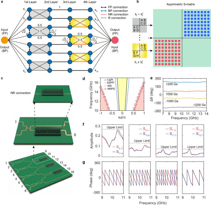
a The 8-input, 8-output deep neural network composed of low-reflection nodes and four types of connections. The network features R and NR connections for bidirectional paths, as well as FP and BP connections for unidirectional paths. b Design strategy of the S-matrix. The S-matrix of the multi-port network is derived from the S-matrices of its constituent units. c Physical implementation of the nonreciprocal computing network using SSPP waveguides. The 8-input, 8-output network is constructed by interleaving cells, each comprising a power divider and connections. NR connections are realized by NRPS. d Simulated dispersion curves. Comparisons of the dispersion curves for light, microstrip (MS), and SSPP waveguides, which highlight the near-field properties of SSPP waveguides. Under a magnetic bias, NRPS exhibits asymmetric forward and backward dispersion. e DPS spectrum under magnetic modulation. The DPS of NRPS varies with the magnitude and direction of the bias magnetic field. f Amplitude spectra of three typical S-parameters. The bidirectional amplitude transmission remains symmetric. g Phase spectra characteristics. The first three processed groups (passing through NRPS) exhibit significant forward-backward splitting, while the fourth group (without passing through NRPS) remains overlapped.
Interestingly, the introduction of nonreciprocity expands the transformation space of the T-matrix of a multi-port network. The T-matrix of the network is mainly obtained by multiplying the sub-matrices of each cell. In reciprocal networks, all connections in cells are subject to the constraint of det (TR) = 1, limiting the overall transformation space. In contrast, for the nonreciprocal networks, this determinant constraint on the connections is lifted, i.e., det (TNR) ≠ 1 (see Supplementary Text 1 for details). Therefore, the nonreciprocity introduced by the connections can add degrees of freedom (DOF) for the design of the T-matrix of the cascaded network, thereby expanding the scope of the transformation space. The enlarged transformation space improves the bidirectional computing performance. In this situation, the S-matrix of the network becomes asymmetric (Fig. 2b), thereby satisfying the prerequisite for independent bidirectional transmission matrices depicted in Fig. 1b. This provides a theoretical basis for bidirectional decoupled propagation in multi-port networks.
To achieve the asymmetric matrix, the NRPS controlled by a static bias magnetic field is utilized. The NRPS in Fig. 2c comprises ferrite, SSPP transmission lines, and a trapezoidal transition structure. Time-reversal symmetry can be broken by the magneto-optical effect, when the spin direction of a circularly polarized field aligns with the magnetic bias in gyromagnetic media. Upon application of an external magnetic field, the dispersion curves for forward and backward waves split as shown in Fig. 2d, with the difference between them defined as the differential phase shift (DPS). To enhance this effect, a pure circularly polarized field is needed40. However, the generation of circularly polarized modes is challenging in ordinary transmission lines. Here, we employ a curved SSPP transmission line to synthesize circularly polarized fields at equidistant points of adjacent wires in Fig. S4a. By periodic arrangement of quasi-TEM cells to introduce a specific phase shift, circular polarization can be formed (in Fig. S4b). Therefore, the magneto-optical effect is enhanced in a minimal area. To demonstrate the effect of curvature on the magneto-optical effect in SSPP waveguides, three different types of SSPP waveguides are compared in Fig. S6. Details are shown in Supplementary Text 2. Unlike surface plasmon polaritons at optical frequencies, SSPPs are artificially structured to operate at microwave frequencies, offering greater design flexibility and frequency scalability43,44 (for more details, see Supplementary Text 3). As shown in Fig. S6, the DPS per unit length along the propagation direction for the large-curved SSPP, weak-curved SSPP, and microstrip line are 11.54°/mm, 4.04°/mm, and 0.22°/mm, respectively. The large-curved SSPP has more obvious nonreciprocity in unit length; thus, the volume of ferrite required is effectively reduced for minimization.
The simulation results of the NRPS are shown in Fig. 2d. The propagation constant of the SSPP waveguide exceeds those in microstrip and optical lines (e.g., 0.88, 0.26, and 0.18, respectively). It thus offers slow-wave and strong confinement characteristics that are beneficial in low-crosstalk miniaturization45. Notably, one design challenge is the mode matching. Due to the high dielectric constant of the substrate, a larger DPS requires an exceedingly narrow SSPP line, posing challenges for interconnection. To address the issue, a gradient-progressive transition structure is thus designed to achieve optimal impedance matching. Further details of this structure can be found in Supplementary Text 4. The DPS of the NRPS can be continuously tuned from 80° to 280° as the static magnetic field increases, as shown in Fig. 2e.
The designed NRPS can be cascaded to a 50:50 power divider (i.e., the R cell), forming the 2-input 2-output NR cell in Fig. 2c. Subsequently, the 8-input 8-output network is constructed using four R and three NR cells, as demonstrated in Fig. 2c. The primarily transmission coefficients of the network are plotted in Fig. 2f, confirming the symmetrical amplitude transmission in FP and BP. Additionally, the transmission coefficients’ amplitudes from port 11 to ports 4, 5, and 7 vary in a step of 6 dB. It originates from the required weights of connections between nodes for balanced and high-efficiency energy transmission among ports. Figure 2g shows the corresponding phase curves of the S-parameters, with their slopes determined by the number of activated BP connections. The bidirectional phase curves in NR cell-integrated channels exhibit a clear split, whereas those in R cell-integrated channels show complete overlap. The fabricated sample of the 8-input 8-output computing network is illustrated in Fig. 3a. As shown in Fig. 3b, the phase curves of S1,11 and S11,1 clearly separate, demonstrating the bidirectional path splitting capability of the sample. As a result, the FP and BP matrices are decoupled, enabling the splitting of bidirectional pathways on a single circuit.
Fig. 3: Experimental results of the nonreciprocal computing network.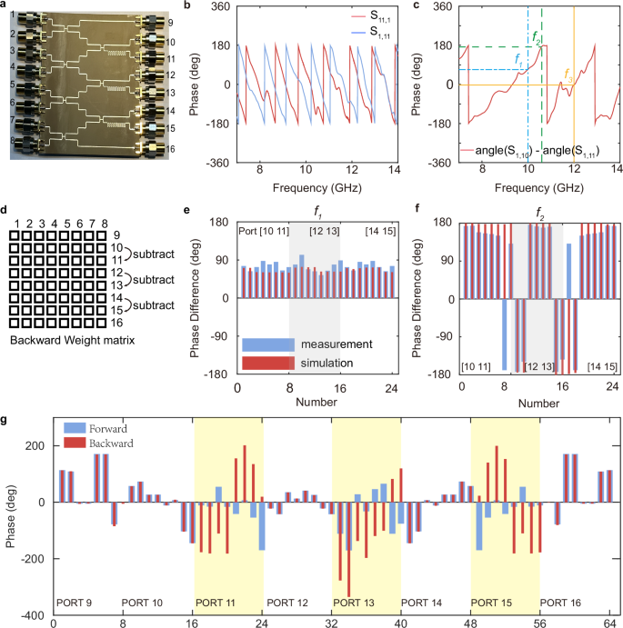
a Image of the fabricated sample. b Phase spectrum of the S-parameters. The phase response in the forward path (S11,1) deviates from the backward one (S1,11) over a broad band. c PD of DCH. The PD can be flexibly tuned from −π to π across a wide frequency band, such as f1 (10 GHz), f2 (10.6 GHz), and f3 (12 GHz). d PD calculation for unidirectional transmission. The PDs for the three DCHs are calculated by subtracting the adjacent rows of the weight matrix. e, f Comparison of PDs in the BP path. The PDs of the three DCHs to ports 1–8 at f1 and f2. The simulated (red) and experimental (blue) data are consistent. g S-parameter’s phase of bidirectional propagation. The S-parameter’s phase from ports 9–16 to ports 1–8 at f2. Processing associated with the NRPS (ports 11, 13, and 15) exhibits a clear difference between forward (blue) and backward (red).
Next, we introduce the performance of the frequency division multiplexing. For the BP path, we define two adjacent ports (e.g., ports 10 and 11) as a differential channel (DCH). The phase difference (PD) from the DCH to the same port (e.g., port 1) varies with frequency, as shown in Fig. 3c. It arises from the differing transmission line lengths in the DCH and is influenced by the magneto-optical effect of the ferrite. This PD reflects the computational function of the DCH, such as addition (0°) or subtraction (180°) operators. Therefore, the function of the DCH changes in a wide frequency range. Three DCHs (ports 10 and 11, ports 12 and 13, and ports 14 and 15) are chosen to be discussed here. Figure 3e, f illustrates the PDs at two frequencies. At 10.6 GHz, the PDs of all three DCHs are ~180°, demonstrating their potential for differential operations. At 10 GHz, the PDs are ~70°, highlighting their potential for orthogonal and integral operations. Moreover, to show the total transmission coefficients between each port, all elements of the forward and backward transmission matrices are presented in Fig. 3g. Among these 64 data points, only the transmission coefficients (highlighted in yellow) related to ports 11, 13, and 15 (passing through the NRPS) differ between the bidirectional directions, reflecting the nonreciprocal effect of the NR cells.
Bidirectional decoupled image processing
To apply the decoupling capability between the FP and BP, we implement structure-based bidirectional decoupled image processing. As shown in Fig. 4, the two unidirectional propagations of the multi-port network have different computational functions. The FP generates a region-integrated image, mimicking global perception in biological neural systems, while the BP performs edge detection, simulating localized response. This confirms that the brain-inspired nonreciprocal neural network effectively realizes integrated perception and response, without the external directional modules.
Fig. 4: Image processing results based on a bidirectional decoupled network.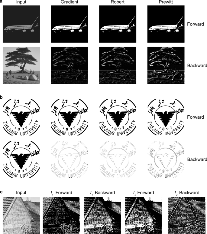
a Image processing results of grayscale images with basic, Robert, and Prewitt operators. The network effectively enhances image contrast and extracts the edge features in the FP and the BP paths, respectively. b Image processing results of binary images. Only the BP path implements edge detection. c Frequency division multiplexing characteristics of the network. In the forward path, the network performs edge detection and image contrast enhanced at f1 and f2, respectively. The backward path is exactly the opposite.
Image processing in the multi-port network is performed by matrix-vector multiplication. We first encode and divide the two-dimensional input image into several 1 × 8 pixel vectors, denoted as Iini = [I1 I2 I3 I4 I5 I6 I7 I8], where I1–I8 is the pixel value of the image. The number of pixel vectors depends on the size of the original image and the encoding method. The 8 elements of a single pixel vector excite the 8 input ports of the network simultaneously in a single operation. Then the measured S-parameters are used to construct the 8 × 8 weight matrix W of the network. Thus, the signal of the output port is O = Iini × W = [O1 O2 O3 O4 O5 O6 O7 O8]. To maximize energy utilization, the output signals of 8 ports are summed as the result of image processing. This is similar to a virtual series connection of 8-in 1-out coupler at the output of the multi-port network, and the output of the virtual coupler is taken as the final output port. To show the process more clearly, the overall transmission matrix K is defined, which describes the transmission coefficient from each input port to the final output port. Each element of K is represented by \({{{{\rm{k}}}}}_{j}={{{{\rm{a}}}}}_{j}\times {e}^{i{\varphi }_{j}}\), which is numerically equal to the sum of the transmission coefficients from port 1 to ports 9–16. As a result, our final output result is R \(={\sum }_{j=1}^{8}{{{{\rm{O}}}}}_{j}={{{{\rm{I}}}}}_{{ini}}\times {{{\bf{K}}}}={\sum }_{j=1}^{8}{{{{\rm{I}}}}}_{j}{{{\boldsymbol{\times }}}}{{{{\rm{k}}}}}_{j}\). Here, j represents the sequential number of the input port. Note that the K varies with frequency within a wide band (see Supplementary Text 5 for details). Leveraging the interleaved cascading topology of the circuit and the phase modulation of NRPS, we can achieve: For the FP path, uniform \({{{{\rm{a}}}}}_{j}\) and \({\varphi }_{j}\) across all ports generate region-integrated images with enhanced contrast. For the BP path, phase modulation of NR cells (e.g., \({{\varphi }_{2}-\varphi }_{3}\approx 180^\circ\)) enables weighted first-order differentiation, producing an edge detection.
Based on the above principles, the image processing for grayscale and binary images is demonstrated through three different operators. For the grayscale image in Fig. 4a, the original image of size 1024 × 1024 in FP has low contrast, with the ratio of the brightest to the darkest pixels being 4.51. After the signal processing by the network, the pixel ratios of the three operators are 7.98, 7.94, and 9.27, respectively. This indicates that forward processing achieves enhancing image contrast, effectively simulating the global perception of the biological systems. For the image of size 256 × 256 in BP of Fig. 4a, the three gradient operators all effectively extract the edges of the original image, indicating backward processing accomplishes edge detection, imitating the backward localized specific response. Interestingly, the images of arbitrary resolution are decoupled and processed in both the forward and backward paths. For a binary image of size 876 × 876 in Fig. 4b, the forward allows image passthrough, while the backward performs edge detection. Moreover, operators can be flexibly adjusted by varying the encoding of the input data (for more details, see Methods). Interestingly, the implementation effects of three edge detection operators vary. Taking the grayscale image as an example, we define edge contrast as the ratio of pixel values between bright and dark areas of edges. The absolute edge contrast for the three operators is as follows: Prewitt (4.37), Robert (1.76), and basic gradient (1.41). It indicates the clarity of image edges: Prewitt operator performs best, followed by the Robert, while the last is basic gradient. This difference comes from the operator itself. Additionally, compared to the basic operator, the edges extracted by the Robert operator are thicker. The Prewitt operator demonstrates the most significant edge extraction effects in both horizontal and vertical directions. However, when the image edges approach ±45°, the Robert algorithm performs better. The difference is due to the operator itself.
Furthermore, to improve image generation quality, the image processing results here are the direct output of a linear digital layer. This linear layer is the weight matrix of the network, projecting the input image onto the final desired output in the digital platform. Compared to direct optical readout, the high-precision computations of digital computers enhance the performance of optical computing hardware. Therefore, by combining the analog and digital domains, the computational power is increased and the burden on digital hardware is alleviated. The development of similar strategies has already become quite mature46.
Bidirectional frequency division multiplexing
The network not only supports nonreciprocal propagation but also features frequency division multiplexing capabilities. Different computational functions can be achieved by varying the frequency. It is shown by the PDs in the DCH transmission coefficients in Fig. 3c. Specifically, at 10.2 GHz, the PD is 86.3°, allowing for orthogonal modulation; at 10.6 GHz, it is −185.5°, enabling differential operations; and at 12 GHz, it is −2.8°, facilitating integral operations. Figure 3d shows that the S-matrix of the network varies with frequency. Multiple asymmetric S-matrices are constructed over a broad frequency range, thus enabling diverse computational functions.
Figure 4c illustrates the bidirectional processing for the original image of size 256 × 256 at two frequencies. Both frequencies use the same encoding method based on the Prewitt gradient operator. At f1, the FP path performs edge detection, while the BP outputs a regional integral image; at f2, the FP outputs an integral image, and the BP conducts edge detection. And the edge extraction capabilities of f2 are different from f1. The edge contrast of the output image at the two frequencies is f1 (2.31) and f2 (3.14), indicating that edges extracted at f2 are clearer. The distinctive is because the PD at f1 is 120°, while at f2 is −185.5°. This makes the operation at f2 closer to the ideal gradient (180°). Overall, both frequencies accomplish integral and gradient operations, but they exhibit completely opposite functionalities in the same propagation direction. Thus, this structure achieves a wide range of nonreciprocal computational functions through frequency division multiplexing, effectively enhancing the versatility of the functions in the perception-response system.
Inverse matrix operation capability through a feedback network
The network can also perform matrix operations by incorporating recursive feedback waveguides, such as matrix solving. As shown in Fig. 5a, the system consists of a computational network, feedback structures, and matched loads. Three waveguides are used to sample input and output signals, while three feedback waveguides introduce recursion. Note that the feedback line lengths are precisely designed to be integer multiple of the wavelength to ensure phase-matching conditions for multi-port inputs. In this case, steady-state recursion is utilized to achieve the Neumann series, which is mathematically equivalent to matrix inversion. This demonstrates that the computing capabilities of the network are scalable with a high level of integration.
Fig. 5: Matrix solver based on a feedback system.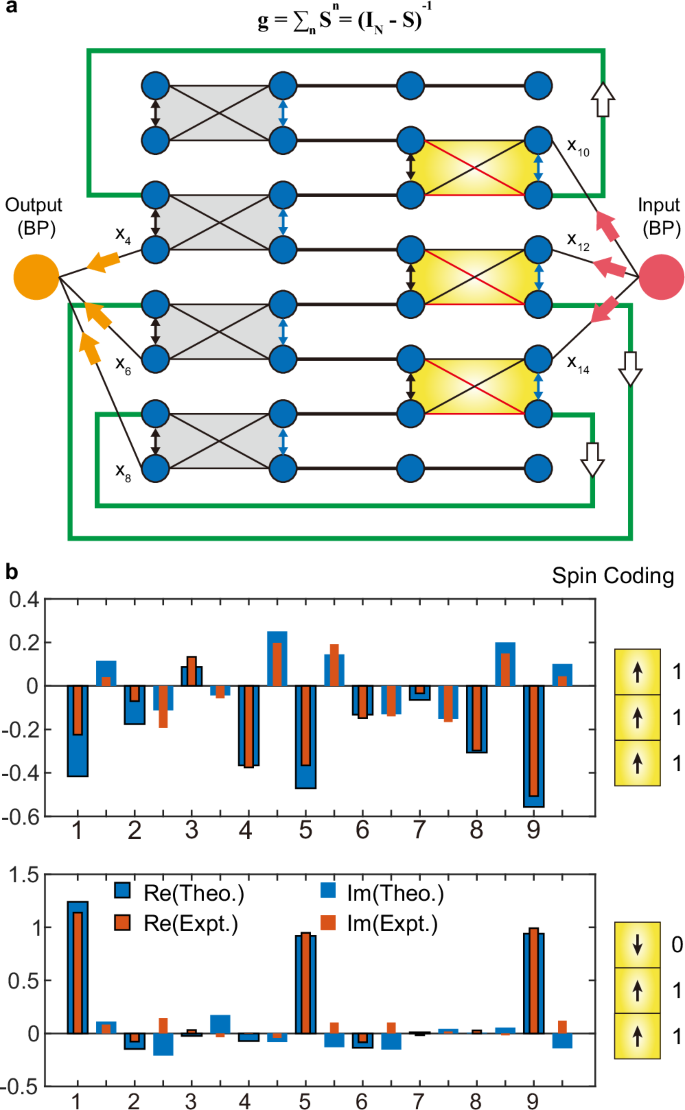
a The closed-loop network for inverse matrix computation. The network consists of three feedback waveguides that connect ports 3 and 11, 5 and 13, 7 and 15, respectively. The feedback waveguides produce recursive wave propagation within the network. Arrows indicate the direction of wave flow through the structure. b Inverse matrix computation results under two spin encoding conditions. The results (nine elements of the 3 × 3 matrix) are extracted from the output port, and the experimental (red) and theoretical (blue) data [real part (boxed) and imaginary part (unboxed)] demonstrate good consistency.
First, to positively design and analyze the feedback system model, the formula representing the transmission of the system is derived. The signal is carried in the form of a complex-valued electromagnetic field, propagating in the recursive path of the system. Both forward and backward recursive paths exist due to the presence of both internal and external connections. Therefore, the output signal is the superposition of the inner and outer loops. We consider typical conditions (eigenvalues of the target matrix being less than one), and the field in the system converges to a steady state. The solution is obtained in this steady state. For instance, for the BP path, the signal is input into the system as shown in Fig. 5a, and the output is:
$${{{{\bf{OUT}}}}}_{{{{\rm{FB}}}}}=\left({{{{{\bf{S}}}}}_{{{{\rm{N}}}}}+{{{\bf{g}}}}}_{{{{\rm{F}}}}}+{{{{\bf{g}}}}}_{{{{\rm{B}}}}}\right)*{{{{\bf{I}}}}}_{{{{\rm{in}}}}}$$
(1.1)
$${{{{\bf{g}}}}}_{{{{\rm{F}}}}}={{{{\bf{S}}}}}_{{{{\rm{N}}}}8}*\left({\sum }_{{{{\rm{n}}}}}{{{{{\bf{S}}}}}_{2}}^{{{{\rm{n}}}}}\right)*{{{{\bf{S}}}}}_{{{{\rm{N}}}}0}$$
(1.2)
$${{{{\bf{g}}}}}_{{{{\rm{B}}}}}={{{{\bf{S}}}}}_{{{{\rm{N}}}}2}*{{{\bf{g}}}}*{{{{\bf{S}}}}}_{0}={{{{\bf{S}}}}}_{{{{\rm{N}}}}2}*\left({\sum }_{{{{\rm{n}}}}}{{{{{\bf{S}}}}}_{1}}^{{{{\rm{n}}}}}\right)*{{{{\bf{S}}}}}_{0}$$
(1.3)
Here, \({{{{\bf{I}}}}}_{{{{\rm{in}}}}}\) is any input signal, and SN, gF and gB represent ground noise, forward recursion, and backward recursion, respectively. Si represents 3 × 3-sized sub-matrices of the S-matrix of the original 8-input 8-output computational network, and the detailed information is shown in the Supplementary Text 6. The series summation corresponds to the matrix inversion, so Eq. (1.3) becomes:
$${{{{\bf{OUT}}}}}_{{{{\rm{E}}}}}=\left({{{{\bf{S}}}}}_{{{{\rm{N}}}}}+{{{{\bf{S}}}}}_{{{{\rm{N}}}}8}*{\left({{{{\bf{I}}}}}_{{{{\rm{N}}}}}-{{{{\bf{S}}}}}_{2}\right)}^{-1}*{{{{\bf{S}}}}}_{{{{\rm{N}}}}0}+{{{{\bf{S}}}}}_{{{{\rm{N}}}}2}*{\left({{{{\bf{I}}}}}_{{{{\rm{N}}}}}-{{{{\bf{S}}}}}_{1}\right)}^{-1}*{{{{\bf{S}}}}}_{0}\right)*{{{{\bf{I}}}}}_{{{{\rm{in}}}}}$$
(1.4)
Therefore, once the scattering matrix is known, the output signal is the inverse matrix modulation operation of any input signal. The theoretical inverse matrix is obtained through noise reduction and de-embedding operations. Note that the inverse matrix operation (\({{{{\bf{g}}}}}_{{{{\rm{B}}}}}\) or \({{{{\bf{g}}}}}_{{{{\rm{F}}}}}\)) represented by the inner loop (\({{{{\bf{S}}}}}_{1}\)) or the outer loop (\({{{{\bf{S}}}}}_{2}\)) can be regarded as the target, and the remaining part (SN + gF or SN + gB) only needs to be removed as noise. It effectively reflects the diverse computational capabilities of the feedback network, as two different inverse matrix operations can be calculated at once. And the steady-state solution for the FP path is similarly presented in the Supplementary Text 6.
Furthermore, unlike traditional feedback-based matrix solvers47, the solvable matrices can be tuned flexibly. As shown in Eq. (1.4), the matrix to be solved is related to the scattering matrix of the initial system. Thus, by modulating the transmission of the nonreciprocal network, the matrix changes accordingly. As discussed in the previous sections, this system features two decoupled unidirectional paths, and the paths are modulated by the ferrite bias magnetic field. Therefore, the matrix-solving capabilities of the feedback network are flexibly controlled by the propagation direction, operating frequency, and ferrite bias orientation. This demonstrates the reconfigurable computational functionality of the network.
To verify the feasibility of matrix inversion, simulations based on Fig. 5a are conducted in CST for the feedback network. To demonstrate the reconfigurable computational capabilities of the network, we encode the spin direction of the ferrite to distinguish different situations. 1 and −1 are used to represent the bias magnetic field direction of the ferrite, where 1 is the y-direction bias and −1 is the −y-direction bias. When the spin codes are set to [1 1 1] and [−1 1 1], the simulations are both basically consistent with the theoretical results, as shown in Fig. 5b. Here, the theoretical solution is based on Eq. (1.4). The specific structure diagram and field map distribution are in the Supplementary Text 7. The Fig. 5b not only verifies the accuracy of the formula, but also verifies the multi-matrix solution capability of the feedback system by the spin code of ferrites.