

In the previous section, the classical data is transformed into a quantum-inspired system as a quantum information system relative to the maximum reference in Table 1 from 2009 to 2019. The first type of state is a 4017 daily pure weather state. The second type of state includes 132 mixed-weather monthly states obtained using square matrices. Hence, the corresponding mathematical model is prepared and the quantum information system is created. The quantum information system is ready to be checked using the quantum informative relations. In this section, the prepared quantum information system is investigated in detail. In the following analysis, we compute the fidelity F, classical information CI, quantum information QI and decoherent information DI, Shannon entropy \(H_{CI}\) of CI, Shannon entropy \(H_{QI}\) of QI, von Neumann entropy \(S_{N}\) of DI, and quantum stability index \(\theta\). The San Francisco weather dataset is presented briefly, accompanied by eight figures for eight variables of the dataset 21. The maximum temperature, minimum temperature, dew point, cloud cover, humidity, precipitation, pressure, and wind speed are plotted versus days in Fig.1. All figures take nearly identical waveforms of distinct amplitudes, except for precipitation. The behavior of the weather variables is nearly regular; otherwise, for precipitation.
Fig. 1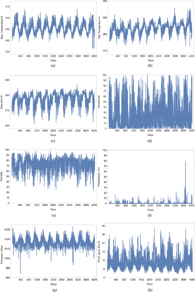
San Francisco weather features. (a) Minimum temperature. (b) Maximum temperature. (c) Dew point. (d) Cloud cover. (e) Humidity. (f) Precipitation. (g) Pressure. (h) Wind speed.
Fidelity
Here, fidelity is used to test the efficiency of the maximal reference in Table 1, by Eq. (5), \(F\left( \left| R_{jk}\right\rangle ,M_{k}\right) =\left\langle R_{jk}\right| M_{k}\left| R_{jk}\right\rangle ,\) where \(\left| R_{jk}\right\rangle\) is the \(j-\)dialy pure state and \(M_{k}\) is the monthly state. We computed the fidelity for 4017 values. Therefore, not all fidelity values can be tabulated here. Therefore, Table 2 is constituted instead of tabulating fidelity values to represent important values where the factor \(F \times 10^{3}\) is applied to all values in the table. Some facts about the years 2009–2019 are displayed.
In the table, days are presented horizontally, while some fidelity values and the number of days that describe fidelity intervals are vertically tabulated for a fixed month. \(F_{\max }\) is the maximal fidelity value per month, \(F_{avg}\) is the average fidelity value per month, \(F_{\min }\) is the minimal fidelity value per month, \(F_{R}=F_{\max }-F_{\min },\) is the fidelity range and \(F_{\sigma }\) is the standard deviation of fidelity. Here, there are six fidelity intervals, and several days are mentioned for the corresponding intervals. Regarding fidelity values, it is eminent that \(F_{avg}\) is closer to \(F_{\max }\) than \(F_{\min }\) despite the large \(F_{R}\) for all years to two intervals [0.8, 0.9) and \(\left[ 0.9,1\right]\), respectively. The fidelity values are generally distributed as 2, 11, 28, 174, 1327, and 2475 in [0, 0.5], (0.5, 0.6), [0.6, 0.7), [0.7, 0.8), [0.8, 0.9), and [0.9, 1], respectively. All values of \(F_{\max }\), and \(F_{avg}\) are located in [0.9, 1] while the values of \(F_{\min }\) are located in [0, 0.5], (0.5, 0.6),[0.6, 0.7), and [0.7, 0.8). The values \(F_{\max }\) do not exceed 0.984 with a minimum value of 0.981. The values \(F_{avg}\) are enclosed between 0.901 and 0.936. The values \(F_{\min }\) take the minimal value 0.472 and the maximal value 0.732. The values \(F_{\sigma }\) are between 0.045 and 0.06. Thus, the interval \(\left[ F_{avg}-F_{\sigma },F_{avg}+F_{\sigma }\right]\) is located between [0.8, 0.9), and [0.9, 1]. Therefore, the major weather data is more coherent with respect to the maximal reference. In Fig. 2, the fidelity is plotted versus the months from January 2009 to December 2019. The fidelity is evident in the waveforms of varying amplitudes. The fidelity ranges between 0.472 and 0.984. Thus, it is notable that the fidelity inspects the maximum weather reference of Table 1. The majority of days have high fidelity values that are greater than 0.8. This maximum weather reference is certainly considered a good reference. Hence, this maximal weather reference can be used to measure other quantum informative relations.
Table 2 Fidelity values of monthly states \(F\times 10^{-3}\), based on years from 2009 to 2019.Fig. 2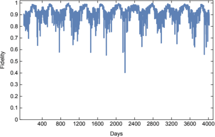 Predictions
In this context, quantum informative measurements are non-linear waveforms. They are numerical values and do not have a functional formula. Consequently, we expect the functional formula for each quantum informative measurement. The Fourier series is an adequate functional formula. Therefore, we expect two Fourier series forms for more accuracy and precision. Let us suppose that the Fourier series consists of a free term, ten cosine terms, and ten sine terms, respectively, expressed as:
$$\begin{aligned} f\left( t\right) =a_{0}+\sum _{j=1}^{10}(a_{j}\cos (\dfrac{j\pi t}{12} )+b_{j}\sin (\dfrac{j\pi t}{12})). \end{aligned}$$
(24)
where \(a_{0},a_{1},a_{2},\ldots ,a_{10},b_{1},b_{2},\ldots ,b_{10}\) are real parameters. The Fourier series parameters are later computed using computational values of quantum informative measurements; CI, QI, DI, \(H_{CI},\) \(H_{QI},S_{N}\) and \(\theta ,\) are found by Eqs. (7–16). The fitting curve method is used as the technique to find the parameters of the Fourier series as follows:
$$\begin{aligned} r=\sum _{k=1}^{N}\left( f\left( t_{k}\right) -f_{k}\right) ^{2}. \end{aligned}$$
(25)
where \(f\left( t_{k}\right)\) is the predicted value at time \(t_k\) and \(f_{k}\) represents the corresponding computed value for the quantum measurement f.
Table 3 Fourier coefficients of \(CI_{p1}, QI_{p1}, DI_{p1}, H_{CIp1}, H_{QIp1}, S_{Np1}, \theta _{p1}\).
The parameters of the first Fourier series are determined by numerical computational values of each quantum informative measurement from January 2009 to December 2017, while the parameters of the second Fourier series are deduced by numerical computational values of the same quantum informative measurement from January 2009 to December 2019. The first and second Fourier series depend on 108 values and 132 values, respectively. Later, we must estimate some future values of quantum informative measurements using two Fourier series. Therefore, the Fourier series can be utilized to predict future month values of the years 2020 and 2021, respectively. The parameters of the first and second Fourier series are tabulated in Tables 3 and 4, respectively, for \(CI_{pj}\), \(QI_{pj}\), \(DI_{pj}\), \(H_{CIpj},\) \(H_{QIpj},S_{Npj}\), and \(\theta _{pj},j=1,2\). Two series are checked comparing with the computational values of quantum informative measurement in three absolute errors; \(E_{1}=\left| q_{c}-q_{p1}\right| ,\) \(E_{2}=\left| q_{c}-q_{p2}\right| ,\) and \(E_{3}=\left| q_{p1}-q_{p2}\right|\), where q is the quantum informative measurement. Also, the Pearson correlation of the three absolute errors is calculated to distinguish between the set of computational values and the two Fourier series to recognize the quality of future predictions.
Table 4 Fourier coefficients of \(CI_{p2}, QI_{p2}, DI_{p2}, H_{CIp2}, H_{QIp2}, S_{Np2}, \theta _{p2}\).Classical information
The classical information values \({CI}_{c}\) of the monthly states are calculated for consecutive months by Eqs. (7, 21, 22, 23) and are listed in Table 5. From 2009 to 2019, \(CI_{c}\) has a minimal value of 0.20261 in August 2015 and a maximum value of 0.40266 in December 2013. Consequently, \(CI_{c}\) ranges between 0.20261 and 0.40266. \(CI_{c}\) generally declines from 2009 to 2019 for all months. From May to October, \(CI_{c}\) is characterized by small values and variations, but in other months, it has large values and variations, especially in January and December. Therefore, the variation of \(CI_{c}\) takes nonlinearly wavily forms of different amplitudes from the maximal value in January to the minimal value in July and August and reaches another maximal value in December every year.
Table 5 Classical information \(CI_c \times 10^{-5}\).
In Table 6, \(P_{C}\left( {CI}_{c},{CI}_{p1}\right) =0.72818\) and \(P_{C}\left( {CI}_{c},{CI}_{p2}\right) =0.73487\) are good correlations, while \(P_{C}\left( {CI}_{p1},{CI}_{p2}\right) =0.99088\) has an excellent correlation. The second correlation provides slightly better results compared to the first prediction. In Table 7, \(E_{3\min }=0.00021\) at Sep/2020 and \(E_{3\max }=0.00803\) at January 2020. \(E_{3\min }=0.00021\) at Sep/2021 and \(E_{3\max }=0.00918\) at Jul/2021. The years 2020 and 2021 behave the same as in previous years. It is evident that \(CI_{c},\) \(CI_{p1}\) and \(CI_{p2}\) have irregular wavily behaviors and vary annular in Fig. 3. Three curves are near for most of the points.
Table 6 Min, Avg, and Max of absolute errors, standard deviation, and Pearson correlation of CI.Fig. 3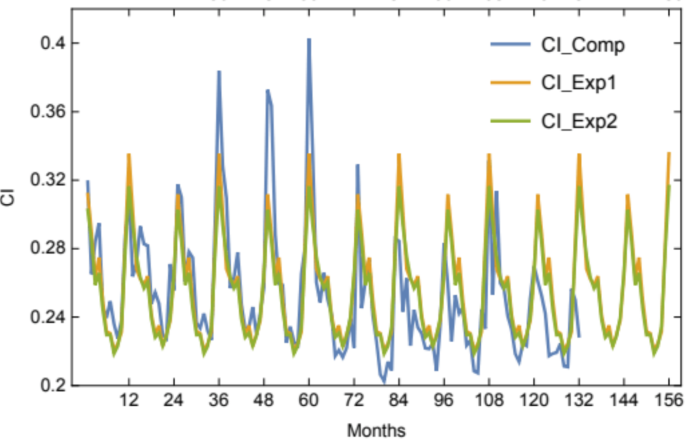
Classical information CI.
Table 7 Predictions of \(CI_p \times 10^{-5}\), for 2020 and 2021.Quantum information
Quantum information QI is checked for monthly states such as CI and \(QI_{c}\) of monthly states, which are also computed for each month by Eqs. (8, 21, 22, 23) and are listed in Table 8. From 2009 to 2019, \(QI_{c}\) ranges between the minimal value of 0.45402 in Dec. 2013 and the maximum value of 0.77238 in Aug. 2015. Clearly, \(QI_{c}\) reaches a maximum in July and August and decreases minimally in January and December based on the annular. Therefore, the variation of \(QI_{c}\) oscillates in nonlinearly sinusoidal forms of different amplitudes from the minimal value in January to the maximal value in July and August and returns to another minimum value in December every year. In regarding of \(CI_{c},\) \(QI_{c}\) behaves inversely behavior of \(CI_{c}.\) If \(QI_{c}\) increases, then \(CI_{c}\) decreases and vice versa. Also, by comparing Tables 5 and 8, \(QI_{c}\) is always greater than \(CI_{c}\) for all months and years. Thus, the effect of \(QI_{c}\) is stronger than the effect of \(CI_{c}\) in this model. Without repetitions, other tables are designed completely as CI tables. In Table 9, the first and the second predictions of \({\small QI}_{p1}\) and \({\small QI}_{p2}\) give excellent results especially \(P_{C}\left( {\small QI}_{c},{\small QI}_{p1}\right) =0.86751\) and \(P_{C}\left( {\small QI}_{c},{\small QI }_{p2}\right) =0.87341.\) Both of \(P_{C}\left( {\small QI}_{c},{\small QI} _{p1}\right)\) and \(P_{C}\left( {\small QI}_{c},{\small QI}_{p2}\right)\) are greater than \(P_{C}\left( {\small CI}_{c},{\small CI}_{p1}\right)\) and \(P_{C}\left( {\small CI}_{c},{\small CI}_{p2}\right) ,\) respectively. In Table 10, the lowest absolute errors are \(E_{3\min }=0.00008\) in March 2020 and \(E_{3\min }=0.00021\) in August 2021. The greatest absolute errors are \(E_{3\max }=0.01200\) at January 2020 and \(E_{3\max }=0.2379\) at Dec/2021. \(QI_{p1}\) and \(QI_{p2}\) have the same behaviors in 2020 and 2021 as in past years. It is obvious that \(QI_{c},\) \(QI_{p1}\) and \(QI_{p2}\) change irregularly in Fig. 4. In particular, \(QI_{c},\) \(QI_{p1}\) and \(QI_{p2}\) occupy opposite positions of \(CI_{c},\) \(CI_{p1}\) and \(CI_{p2}\).
Table 8 Qunatum information \(QI_c \times 10^{-5}\).Table 9 Min, Avg, and Max of absolute Errors, standard Deviation, and Pearson Correlation of QI.Fig. 4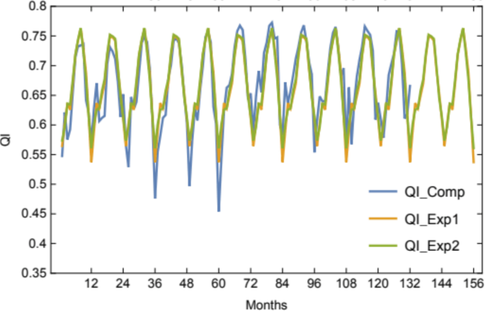 Table 10 Predictions of \({QI}_{p} \times 10^{-5}\).Decoherent information
In this subsection, the decoherent information DI is discussed in addition to the aforementioned CI and QI. In a similar way, \(DI_{c}\) values of monthly states are also computed by Eqs. (10, 21, 22, 23) for all months and are listed in Table 11. A range of \(DI_{c}\) lies between the minimal value of 0.00992 in August 2011 and the maximum value of 0.16884 in February 2019 from 2009 to 2019. There is a near similarity between \(DI_{c}\) and \(CI_{c}\), where \(DI_{c} for the same month. Similarly, other tables are formed with the same techniques of CI and QI.
Table 11 Decoherent information \(DI_c \times 10^{-5}\).Table 12 Min, Avg, and Max of absolute errors, standard deviation, and Pearson correlation of DI.Fig. 5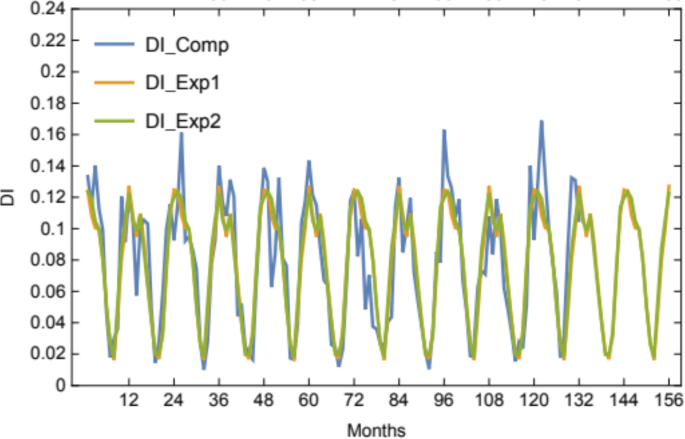
Decoherent information DI.
In Table 12, the second prediction \(DI_{p2}\) gives more accurate results that are distinguishable from the first prediction \(DI_{p1}\) with less absolute errors. Also, \(P_{C}\left( DI_{c},DI_{p2}\right) =0.86597\) and \(P_{C}\left( DI_{c},DI_{p1}\right) =0.87296\) are excellent correlation results such that \(P_{C}\left( DI_{c},DI_{p2}\right) >P_{C}\left( DI_{c},DI_{p1}\right)\) with a slight difference since \(P_{C}\left( DI_{p1},DI_{p2}\right) =0.99200\). \(P_{C}\left( DI_{c},DI_{p2}\right)\) and \(P_{C}\left( DI_{c},DI_{p1}\right)\) are very close to \(P_{C}\left( {\small QI}_{c},{\small QI}_{p1}\right)\) and \(P_{C}\left( {\small QI}_{c},{\small QI}_{p2}\right) ,\) respectively. Hence, the predictions of QI and DI are better than the predictions of CI. In Table 13, the lowest absolute errors are \(E_{3\min }=0.00107\) in March 2020 and \(E_{3\min }=0.00008\) in January 2021. The greatest absolute errors are \(E_{3\max }=0.00512\) in December 2020 and \(E_{3\max }=0.1088\) in February 2021. \(QI_{p1}\) and \(QI_{p2}\) move in the same direction in 2020 and 2021 as in previous years. Eminently \(DI_{c},\) \(DI_{p1}\) and \(DI_{p2}\) curves behave geometrically \(QI_{c},\) \(QI_{p1}\) and \(QI_{p2},\) respectively but differ in computational ranges in Fig. 5.
Table 13 Predictions of \(DI_p \times 10^{-5}\), for 2020 and 2021.Shannon entropy of CI
The purpose of Shannon entropy is to measure the randomness of CI. Therefore, the Shannon entropy values \(H_{CI}\) are determined for monthly states by Eqs. (14, 21, 22, 23) for each month and are recorded in Table 14. From 2009 to 2019, \(H_{CI}\) has the lowest randomness value of CI with 0.57329 in December 2013, and the highest randomness value appears in October 2016 with 0.78533. Hence, \(H_{CI}\) here takes a range between 0.57329 and 0.78533.
Table 14 Shannon entropy of CI \(H_{CIc} \times 10^{-5}\).
For the same month, \(H_{CI}\) often varies with small changes from year to year. October occupies the first month of randomness of CI and is followed by June. Clearly, \(H_{CI}\) oscillates in the same year. It is noted that \(H_{CI}\) increases starting in 2016. Generally, the randomness of CI is considered high. In Table 15, the minimum, average and maximum absolute errors are suitable, as well as the standard deviations. For Pearson correlation, the results are not good where \(P\left( H_{CIc},H_{CIp1}\right) =0.57369\) and \(P\left( H_{CIc},H_{CIp2}\right) =0.58279.\) Consequently, the predictions are not strong and are mean. In Table 16, two predictions \(H_{CIp1}\) and \(H_{CIp2}\) are mentioned for 2020 and 2021. \(E_{3\min }=0.00053\) at Sep/2020 and \(E_{3\max }=0.00870\) at Feb/2020. \(E_{3\min }=0.00050\) at Jul/2021 and \(E_{3\max }=0.02186\) at Dec/2021. In Fig.6, \(H_{CIc},\) \(H_{CIp1}\) and \(H_{CIp2}\) take nonlinear waveforms but the \(H_{CIc}\) curve grows up starting from 2016. The randomness of CI gradually increases in the nonlinear waveform from 2016 to 2019.
Table 15 Min, Avg, and Max of absolute errors, standard deviation, and Pearson correlation of \(H_{CI}\).Fig. 6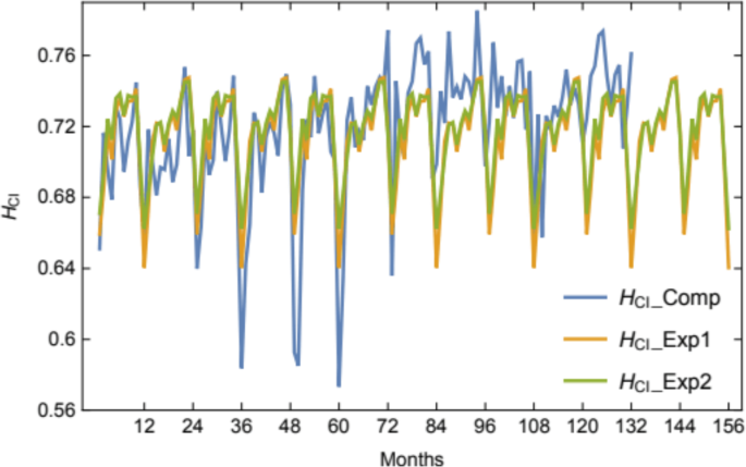
Shannon entropy \(H_{CI}\).
Table 16 Predictions of CI \(H_{CIp} \times 10^{-5}\), for 2020 and 2021.Shannon entropy of QI
In the same way, the Shannon entropy is used to inspect QI similar to CI in the previous subsection. Shannon entropy values \(H_{QIc}\) of monthly states are calculated for each month by Eqs. (15, 21, 22, 23) and are listed in Table 17.
Table 17 Shannon entropy \(H_{QIc}\) of QI.
Obviously, all terms of \(H_{QIc}\) are greater than one since some nondiagonal terms are 72 terms greater than the number of dimensions of the quantum feature space. From 2009 to 2019, a range of \(H_{QIc}\) is located between the minimal value of 2.590 in December 2013 and the maximal value of 4.663 in February 2019. In fact, \(H_{QIc}\) is similar to \(H_{CIc}\) with different ranges. In Table 18, the absolute errors are close to the standard deviations. Two Pearson correlations are weak where \(P\left( H_{QIc},H_{QIp1}\right) =0.40453\) and \(P\left( H_{QIc},H_{QIp2}\right) =0.46559.\) Also, \(P\left( H_{QIp1},H_{QIp2}\right) =0.86890\) is less than \(P\left( H_{CIp1},H_{CIp2}\right) =0.98439.\) It is prominent that predictions of randomness \(H_{QIp1}\) and \(H_{QIp2}\) are not accurate. In Table 19, two predictions \(H_{QIp1}\) and \(H_{QIp2}\) are recorded for 2020 and 2021. \(E_{3\min }=0.015\) at Sep/2020 and \(E_{3\max }=0.221\) at Dec/2020. \(E_{3\min }=0.00001\) at Jun/2021 and \(E_{3\max }=0.297\) at January 2021. In Fig.7, \(H_{QIc},\) \(H_{QIp1}\) and \(H_{QIp2}\) curves are similar to \(H_{CI}\) curves geometrically with different ranges. Consequently, curves of \(H_{CI}\) and \(H_{QI}\) behave physically.
Table 18 Min, Avg, and Max of absolute errors, standard deviation, and Pearson correlation of \(H_{QI}\).Fig. 7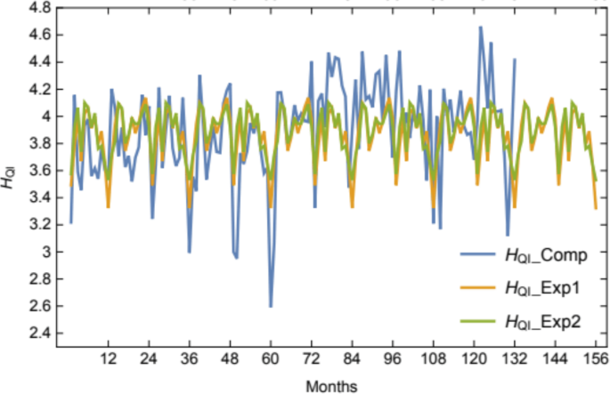
Shannon entropy \(H_{QI}\) based on months.
Table 19 Predictions of \(H_{QIp}\), for 2020 and 2021.Von Neumann Entropy of DI
von Neumann entropy \(S_{N}\) deals with the decoherent information DI to measure its randomness. \(S_{N}\) values of the monthly states are computed for each month by Eqs. (16, 21, 22, 23) and are listed in Table 20. As shown in the table, \(S_{N}\) varies from the lowest value of 0.01717 in August 2011 to the highest value of 0.17635 in February 2011. January and December have the highest von Neumann entropies, while July has the lowest von Neumann entropy. In Table 21, the absolute errors and standard deviations are very small relative to other measurements of quantum information. In addition to the strong correlation between the computational data \({\small S}_{Nc}\) and the predicted data \({\small S}_{Np1}\) and \({\small S} _{Np2}\). The Pearson correlation is strong with values such as \(P\left( {\small S} _{Nc},{\small S}_{Np1}\right) =0.87848,\) \(P\left( {\small S}_{Nc},{\small S} _{Np2}\right) =0.88684,\) and \(P\left( {\small S}_{Np1},{\small S} _{Np2}\right) =0.99057.\) Therefore, two predictions are more accurate in Table 22. \(E_{3\min }=0.00046\) in March 2020 and \(E_{3\max }=0.00674\) in April 2020. \(E_{3\min }=0.00006\) in May 2021, and \(E_{3\max }=0.1481\) in October 2021. In Fig.8, \(S_{Nc},\) \(S_{Np1}\) and \(S_{Np2}\) curves are near to CI curves computationally and geometrically. Hence, \(S_{N}\) and CI coincide in physical characteristics.
Table 20 Von Neumann entropy of DI \(S_{Nc} \times 10^{-5}\).Table 21 Min, Avg, and Max of absolute errors, standard deviation, and Pearson correlation of \(S_N\).Fig. 8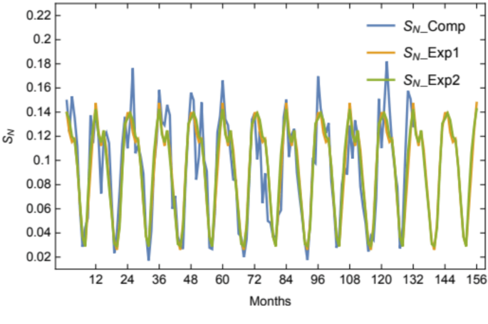
Von Neumann entropy \(S_{N}\).
Table 22 Predictions of \(S_{Np} \times 10^{-5}\) for 2020 and 2021.Quantum Stability Index
The quantum stability index (QSI), denoted by \(\theta\), is introduced mathematically in Sect. “Quantum model of dataset” as a novel quantum informative metric. QSI is a new formula that is defined here to assess the stability of the quantum information system. QSI is designed in terms of three distinct information types; CI, QI, and DI. QSI quantifies the stability by analyzing the relationship among CI, QI, and DI as previously discussed. QSI generally discusses four physical situations for the stability of the quantum information system. The first situation describes the full stable quantum information system when \(\theta =0\). The second situation expresses the stable quantum information system when \(0< \theta < 45^{\circ }\). In the third situation, the quantum information system becomes ambiguous for \(\theta = 45^{\circ }\). No one can say that the system is metastable. When \(45^{\circ } < \theta \le 90^{\circ }\), the fourth situation illustrates that the quantum information system begins to lose stability when \(\theta\) travels away \(45^{\circ }\). The values of the quantum stability index of the monthly states are evaluated in degrees for individual months by Eqs. (13, 21, 22, 23), and are listed in Table 23. For a lot of details about the quantum stability index, it has been inspected for months.
Table 23 Quantum stability index \({\theta }_{c}\).
The quantum stability index \(\theta\) changes from minimal to maximal limits. For example, it increased from 5.72 in August 2011 to 24.26 in February 2019. For the same month, \(\theta\) appears in oscillating forms and varies yearly. The months: January, February, November, and December have the highest variance. In contrast, July and August have less variance. Years change in irregular sinusoidal forms. All terms of \(\theta\) are less than 45 with a difference of 20.74 at least and extending to 39.28. In Table 24, the average absolute errors approach the minimal absolute errors while diverging for the maximal absolute errors. Standard deviations and average absolute errors form suitable intervals of the stability as \(\left[ 0.45,3.13\right]\) and \(\left[ 0.47,2.97\right]\) for \(\theta _{c-p1}\) and \(\theta _{c-p2}\) respectively. Pearson correlations are very strong where \(P\left( \theta _{c},\theta _{p1}\right) =0.88552,\) \(P\left( \theta _{c},\theta _{p2}\right) =0.89691,\) and \(P\left( \theta _{p1},\theta _{p2}\right) =0.98730.\) In Table 25, \(E_{3\min }=0.11\) in September 2020 and \(E_{3\max }=1.27\) in April 2020. \(E_{3\min }=0.07\) in May 2021 and \(E_{3\max }=1.65\) in September 2021. In Fig. 9, \(\theta _{Nc},\) \(\theta _{Np1}\) and \(\theta _{Np2}\) curves look like all quantum informative measurements in nonlinear waveforms. Three curves are very close to the major points.
Table 24 Min, Avg, and Max of absolute errors, standard deviation, and Pearson correlation of \(\theta\).Fig. 9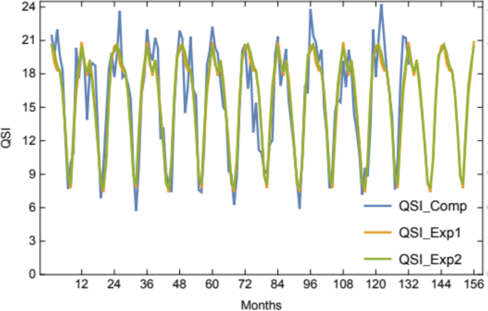
Quantum stability index in degree \(\theta\).
Table 25 Predictions of \(\theta _p\), for 2020 and 2021.Results and analysis
We provide a brief overview of the San Francisco weather model, which is processed using quantum information theory. The classical information system is transformed into a quantum-inspired system using the maximal reference and Euclidean norm to form daily pure and monthly mixed states. The pure daily states of each month are treated with the same monthly state in fidelity to measure the quality of the weather. Most days give excellent results with high fidelity greater than 0.8, especially in July and August from 2009 to 2019. Compared to January and December in the same interval, their fidelity values are smaller. According to the strength effect, three types of information are organized: quantum information, classical information, and decoherent information. Two predictions of QI and DI are close to their computational values because Pearson correlations are excellent. For CI, Pearson correlations are good and the two corresponding predictions are good results. Every type of entropy takes the same arrangement as the type of information. The Shannon entropy of CI is given by nine terms expressing diagonal elements of the state \(\rho\) and is always less than one. The Shannon entropy of QI is described by 72 terms that express non-diagonal elements of the state \(\rho\) and are always greater than one. Two predictions of the Shannon entropy of CI and QI are moderate because the Pearson correlations are moderate and weak. For von Neumann entropy, the Pearson correlations are strong, and the two predictions yield excellent results. In the end, the quantum stability index measures the stability of the quantum information system. It confirms that the instability limit is so far. In contrast. It is more stable. Hence, the weather in San Francisco is moderate from 2009 to 2019 with computational data and continues to moderate from 2020 to 2021 using predictions.