Quantification of record-breaking subsidence in California’s San Joaquin Valley

Methods 1: calculating Valley-wide subsidence volume for 2006–2010Dataset 1

First, we digitized the displacement contours of June 2007–December 2010 subsidence from Fig. 1 of19. For calculating the Valley-wide subsidence volume, we worked directly with these contours, integrating within each contour to obtain the Valley-wide subsidence volume. We used the qGIS “add geometry attributes” algorithm to calculate the areas37. The area of each contour and corresponding subsidence volumes are reported in Supplementary Table 1. We rounded the final cumulative total of 1.15 km3 to 1.2 km3 to account for the approximations involved in the digitization process.

When using the dataset of Farr et al.19 for general mapping of the subsidence, as well as generation of experimental variograms (see “Methods 5” section), we replaced the regions where no subsidence was measured with values from a normal distribution with mean 1 inch and variance 1 inch. This represents that these areas were under the detection threshold of the instrument. (We assume a detection threshold of 2 inches, as this is the smallest subsidence value shown by ref. 19).

Dataset 2

We downloaded the pixel-level December 2006 – January 2010 subsidence data from the repository at ref. 38. We clipped the dataset to only the San Joaquin Valley, projected the average subsidence rates from satellite line-of-sight to vertical by assuming all motion was in the vertical direction and multiplied the pixel values by 3.1 to obtain values of total subsidence for December 2006 – January 2010. We then generated subsidence contours at the same subsidence values as in Dataset 1, and used the qGIS “add geometry attributes” algorithm to calculate the area within each contour37. The area of each contour and corresponding subsidence volumes are reported in Supplementary Table 2. We rounded the final cumulative total of 0.69 km3 to 0.7 km3 to account for the approximations involved in the process.

Dataset 3

First, we digitized the displacement contours of January 2008–2010 subsidence from Figure 17 of ref. 10. For calculating the Valley-wide subsidence volume, we worked directly with these contours, integrating within each contour to obtain the Valley-wide subsidence volume. We used the qGIS “add geometry attributes” algorithm to calculate the areas37. The area of each contour and corresponding subsidence volumes are reported in Supplementary Table 3. We rounded the final cumulative total of 0.73 km3 to 0.7 km3 to account for the approximations involved in the digitization process.

Methods 2: calculating Valley-wide subsidence volume from TRE Altamira dataset

The TRE Altamira dataset contains measurements of vertical motion made every 6 days. To calculate Valley-wide subsidence volume from this dataset, we first created differential subsidence maps by taking the pixelwise difference between adjacent pairs of 6-day separated InSAR images. We then interpolated these differential subsidence maps into a regular, smooth grid by averaging all pixels within a 2 km search radius. This filled most holes in the dataset without overly smoothing the data. Once the data were in regular grid format, we created cumulative subsidence maps by summing the interpolated differential subsidence grids. Finally, we used the “grdvolume” function from the Generic Mapping Toolbox39 to spatially integrate the total volume of subsidence at each 7-day separated grid. We started in May 2015, which was the earliest date to have near-complete coverage of the Valley. An animation showing the evolution of cumulative deformation over time is provided in Supplementary Movie 1.

Methods 3: interpolating between GNSS measurements using inverse distance weighting

We downloaded GNSS measurements for all stations in the United States from the Nevada Geodetic Laboratory40, then filtered the stations to only include those with data spanning the full 2011–2015 period and located in the San Joaquin Valley. We then used the Generic Mapping Toolbox function “nearneighbor” to interpolate between these stations39. We applied a 60 km search radius, meaning any stations more than 60 km from a point did not contribute to the interpolated value at that point. We imposed a restriction that pixels must average at least three measurements and a NaN value would be given if there were fewer than three measurements within 60 km. (We selected the 60 km search radius manually, after finding by trial and error that a smaller radius gave incomplete coverage with lots of NaN values and a larger radius resulted in an unnecessarily smoothed surface). To reduce directional bias, in the situation where there were a) more than three measurements within 60 km and b) two or more of these measurements fell in the same sector (where we defined 360 sectors each of 1 azimuthal degree angular width around the pixel of interest), only the nearest value in each sector was used in the interpolation.

Methods 4: identification of correlation structures in 2006–2010 and 2015–2022 subsidence maps

We extracted the correlation structures from the subsidence maps by first generating experimental variograms and then fitting an ellipse model to them. To generate the experimental variograms, we used the SciKit GStat Python library41. For both the 2006–2010 and 2015–2022 periods, the parameters for variogram generation were: 12 lag distances, evenly spaced between 0 and 110 km; and 8 directions, spaced at 22.5 degrees and with a tolerance of 22.5 degrees. These parameters were chosen to ensure a satisfactory number of datapoints per lag (the number of datapoints per lag is shown in Supplementary Figs. 2 and 3) while also giving good coverage of directions and distance. Note that the number of data in each direction is a function primarily of the Valley geometry, hence the high similarity between Supplementary Figs. 2 and 3.

To fit ellipses (defined by three parameters: azimuthal angle, major axis length and minor axis length) to the variograms, we started with an initial guess for the ellipse parameters, obtained by visual inspection of the experimental variograms. We then manually tweaked the parameters until a good fit, determined by visual inspection, was obtained. In determining a good fit, we placed particular emphasis on matching the model to the short-distance lags, as this is good practice42. The resulting fits to directional variograms are shown in Supplementary Figs. 4 and 5 for 2006–2010 and 2015–2022 respectively. Note that a zonal anisotropy was present in all cases, with the sill showing a directional dependency. We accounted for this using a nested structure in the minor direction with infinite range, following the method for approximating zonal anisotropy described in ref. 43. The best-fitting ellipses are displayed in Fig. 4.

Methods 5: extracting correlation structures for low/no, moderate, and severe drought periods

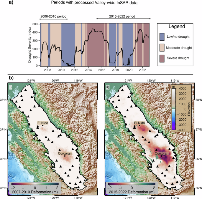
To quantify drought, we used the US Drought Monitor’s Drought Severity and Coverage Index (DSCI) for the region represented by hydrologic unit code 2 – this is a watershed with a boundary that closely approximates the state border of California. We considered the whole of the state because, although this study focuses on the San Joaquin Valley, the hydrology of the Valley is strongly influenced by conditions elsewhere in the state due to the high levels of water deliveries from elsewhere in the state. We note that the San Joaquin River index, a more local index specific to the study area, showed very similar patterns (Supplementary Fig. 1). We set thresholds corresponding to low/no drought, moderate drought and severe drought. The thresholds we used for the three periods were DSCI < 150 for low/no drought, 150 ≤ DSCI < 300 for moderate drought and DSCI > 300 for severe drought. These thresholds were selected so as to match with qualitative information on the history of droughts in California described by various publications44,45 – for instance, both our choice of thresholds and the literature describe the periods 2014-2016 and 2021-2022 as severe drought, and the years 2017 and 2019 as low/no drought.

We defined periods of low/no, moderate, and severe drought as described in “Online Methods 1”. We then generated experimental variograms and fitted 2-D variogram models to the InSAR data corresponding to these three categories. For the 2006–2010 period, the only reliable subsidence data we had were for the span of the entire period, and we treated that period as one of moderate drought intensity, although noting that 35% of that time period fell into the low drought category. For 2015–2022, we had InSAR data with 6-daily resolution. We therefore extracted sub-periods from that data corresponding to the three different categories of drought intensity, omitting periods shorter in duration than 30 days. The extracted sub-periods were:

May 2015 – Oct 2016: severe

Feb 2017 – June 2018: low/no

July 2018 – Jan 2019: moderate

Feb 2019 – Aug 2020: low/no

Aug 2020 – Apr 2021: moderate

Apr 2021 – December 2022: severe

We combined the subsidence totals for each drought category, creating three maps that corresponded to the total subsidence accumulated during periods of low/no drought, moderate drought and severe drought. These maps are shown in Supplementary Fig. 6.

We finally formed experimental variograms and variogram models corresponding to maps for each drought category. Our methodology to generate experimental variograms and fit models was identical to that described in “Methods 5” section, repeated here for clarity:

We extracted the correlation structures from the subsidence maps by first generating experimental variograms and then fitting an ellipse model to them. To generate the experimental variograms, we used the SciKit GStat Python library41. For both the 2006–2010 and 2015-2022 periods, the parameters for variogram generation were: 12 lag distances, evenly spaced between 0 and 110 km; and 8 directions, spaced at 22.5 degrees and with a tolerance of 22.5 degrees. These parameters were chosen to ensure a satisfactory number of datapoints per lag (shown in Supplementary Figs. 7–9) while also giving good coverage of directions and distance. Note that the number of data in each direction is a function primarily of the Valley geometry, hence the high similarity between Supplementary Figs. 7–9.

To fit ellipses (defined by three parameters: azimuthal angle, major axis length, and minor axis length) to the variograms, we started with an initial guess for the ellipse parameters, obtained by visual inspection of the experimental variograms. We then manually tweaked the parameters until a good fit was obtained. In determining a good fit, we placed particular emphasis on matching the model to the short-distance lags, as this is good practice42. The resulting fits directional variograms are shown in Supplementary Figs. 10–12. Note that a zonal anisotropy was present in all cases, with the sill showing a directional dependency. We accounted for this using a nested structure in the minor direction with an infinite range, following the method for approximating zonal anisotropy described in ref. 43. The best-fitting ellipses are displayed in Fig. 4.

Methods 6: kriging between 2011-2015 GNSS measurements

We used the Stanford Geostatistical Modeling Software (SGeMS) to apply the kriging interpolation46. For both nested structures, we specified the major axis length, minor axis length and azimuth in the ordinary kriging algorithm within the software, with a minimum and maximum number of conditioning values set to be one and thirty respectively. We then exported the output as a csv file and reformatted it into grids which could be readily plotted and analyzed using Python. We did this for each of the five correlation structures displayed in Fig. 4.

Methods 7: processing leveling survey and extensometer dataExtensometer data

We first collated information on all extensometers in the San Joaquin Valley. Information on extensometers was sourced from (1) the USGS’s California Water Science Center (https://ca.water.usgs.gov/land_subsidence/central-valley_extensometer-data.xlsx)), (2) the Central Valley Hydrologic Model47, and (3) data reported from the historic period2. From this information, we then identified the five extensometers for which measurements were made for the full 2011–2015 period. These five extensometers were all operated by the USGS, and we used the measurements as available on their online portal. (The data can also be found tabulated alongside the Central Valley Hydrologic Model48). To convert the measured compaction over the extensometer depth interval (cmeas) into total subsidence, we used the empirical relationship between the extensometer depth (d) and the percentage of total subsidence recorded (pctot) developed for the historic period4, which is reproduced below:

$${{pc}}_{{tot}}=133\,{\log }_{10}\left(d\right)-341$$

where it is noted that depth in the above equation is in units of feet, not meters. From this relationship, the total subsidence (stot) at a given extensometer can be estimated as:

$${s}_{{tot}}=\frac{{{pc}}_{{tot}}}{100}* {c}_{{meas}}$$

The estimate of total subsidence obtained using this method is only approximate, since it relies on an empirical relationship from the historic period that may have altered for the recent period, and the r2 value for the relationship in the historic period was relatively low, at 0.764. However, it was sufficient for our purpose of comparing general patterns of subsidence.

Leveling data

Details on the available leveling surveys in the San Joaquin Valley is provided in the Supplemental Material of ref. 30. Of the available surveys, two contain information on the 2011–2015 period: the San Joaquin River Restoration Partners Geodetic Control Network, operated by the Bureau of Restoration; and the monitoring program along the California Aqueduct, undertaken by California Department of Water Resources. Various other programs of leveling surveys have operated in the San Joaquin Valley, but these did not cover the relevant 2011–2015 period.

The leveling survey measurements plotted in Fig. 6 were downloaded from48. We show the measured subsidence at survey points between July 2012 and July 2015 from the San Joaquin River Restoration Partners Geodetic Control Network and the measured subsidence between June 2009 and February 2015 along the California Aqueduct. The measurements are plotted directly (unscaled) in Fig. 6. For the California Aqueduct, only every 5th point is plotted because the raw measurements are spaced ~50 m apart which was too spatially dense for visual display.

Methods 8: obtaining rates and totals for historic subsidence

First, we digitized the cumulative subsidence volume totals from Figures 19, 29, and 38 of ref. 2. This gave totals from 1945 to 1968 for the three subregions of Tulare-Wasco, Kettleman-Los Banos and Arvin-Maricopa. We summed the totals from the subregions to obtain the Valley-wide total, which we show in Supplementary Fig. 12.

To estimate the maximum rate during the historic period, we took the record shown in Supplementary Fig. 12, applied a 3-year smoothing and calculated the maximum gradient. The resulting value was 0.78 km3/year in 1961–62. The average rate was computed by dividing the total subsidence volume by the number of years.