
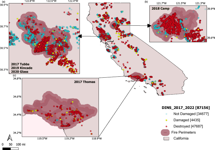
We primarily relied on a modified database from five selected fires that includes more than 47,000 structures with two broad damage states: “Survived” and “Destroyed”, and five detailed damage states: “Destroyed (>50%)”, Damaged (“Major (26–50%)”, “Minor (10–25%)”, “Affected (1–9%)”), “No Damage”. The CAL FIRE Damage INSpection Program (DINS) was founded with the goal to collect data on damaged, destroyed, and unburned structures during and immediately after fire events to assist in the recovery process, and to provide local governments and scientists information for analyzing why some structures burned and why some survived43. Through a public records request, we acquired DINS data for more than 90,000 structures that survived, were damaged, or were destroyed across all California wildfires from 2013–2022, making this potentially the largest combined dataset of its sort. We then incorporated risk factors associated with structure destruction by wildfires to the DINS data to gain a deeper understanding of WUI destruction. These factors include structure density, building materials, year built, defensible space, and exposures to structures (fire intensity and ember). We employed several Machine Learning (ML) techniques to identify and highlight the important features in our WUI data. These techniques included feature selection, feature engineering, and model interpretation methods to ensure we could pinpoint the most influential variables influencing our results. To enhance the performance of the ML model in this study, we implemented a range of data preprocessing techniques such as data cleaning, normalization, and encoding. These preprocessing steps were crucial for improving model accuracy, reducing noise, and ensuring the robustness of our findings. By meticulously preparing the data, we ensured that the ML model could effectively learn and make accurate predictions from our complex WUI dataset. We opted for the XGBoost (eXtreme Gradient Boosting) algorithm for our ML model due to its superior performance over other methods on our dataset. We also leveraged the SHAP (SHapley Additive exPlanations) model, which provides a nuanced understanding of each column’s contribution to the overall predictive outcome. This technique allowed for a comprehensive assessment of the importance of variables within the dataset, enhancing the robustness and reliability of our analysis. The results of Confusion Matrices and Receiver operating characteristics (ROC) Curves, in addition to an advanced computational framework, allowed us to delve into the intricacies of the dataset, capturing complex relationships and patterns that might not be discernible through conventional methods. Our evaluation extended beyond a generalized assessment, as we calculated the accuracy and sensitivity metrics for each individual fire and aggregated the results to encompass all structures within the damage dataset. This meticulous analysis not only provided insights into the predictive performance of our model on a per-fire basis but also yielded a comprehensive understanding of its effectiveness across the entire spectrum of structures in the damage data.
Risk factors to structures from wildfires in the WUI
The methodology for integrating risk factors related to structure destruction builds upon the combination of on-the-ground data with fire modeling reconstructions by Hakes and Theodori et al.34 for community-level risk assessment for the Tubbs fire, which includes:
Structure spacing which represents “Structure Separation Distance (SSD)”. We employed the Microsoft Maps dataset (available at https://github.com/microsoft/USBuildingFootprints), which encompasses open building footprints datasets for entire counties in the United States. This dataset comprises 129,591,852 computer-generated building footprints. Additionally, we utilized QGIS software to access geospatial data concerning urban infrastructure, building locations, and their spatial interconnections.
The year built refers to the year in which the primary structure on a parcel of land was constructed. In the context of analyzing the impact of WUI fires, the Year Built variable is important because the age of a structure can influence its susceptibility to fire damage. Furthermore, it acts as a confounding variable that can affect both the building features and the extent of damage.
Concerning fire safety in building construction materials, numerous in-depth studies have been carried out through meticulously planned laboratory tests18,44. Despite the solid laboratory evidence, few empirical studies have documented building characteristics associated with structure loss in real wildfire situations28. In this study building characteristics include eaves, vent screens, exterior siding, roof construction, and window panes.
In terms of defensible space, which is representing in this study as “Vegetation Separation Distance (VSD)”, the state of California requires fire-exposed homeowners to create a minimum of 30 m (100 ft) of defensible space around structures, and some localities are beginning to require at least 60 m (200 ft) in certain circumstances26. We established three categories for the Vegetation Separation Distance (VSD): Zone0, which comprises the initial five feet from the building or “0–5”; Zone1, encompassing the area within 30 feet of the building or “5–30”; and Zone2, extending to within 100 feet of the building or “30–100” (CAL FIRE DSpace: https://www.fire.ca.gov/dspace). Remote sensing techniques were utilized to analyze the density and distribution of vegetation in the WUI regions and urban settings, extracting valuable insights from the aerial and satellite imagery and LiDAR data. The publicly available datasets (including countywide LiDAR data and a fine scale vegetation and habitat map) which were produced by the Sonoma County Agricultural Preservation and Open Space District and the Sonoma County Water Agency, provide an accurate, up-to-date inventory of the county’s landscape features, ecological communities and habitats (Sonoma County Vegetation Map: https://sonomavegmap.org/).
Exposures including fire intensity (flame length) and firebrand (ember load). Houses are destroyed during wildfires when exposed to flames in adjacent fuel, radiant heat from nearby fuel (≤40 m)16, or airborne embers and firebrands originating in nearby and distant fuel (typically < 10 km)45,46. In this study, we used the Eulerian Level set Model of FIRE spread, ELMFIRE, an operational fire behavior and spread simulation tool35 for its additional capability in simulating ember deposition of multiple embers and its implementation of Monte Carlo analysis36 to capture the stochasticity and uncertainty inherent in wildland fire modeling. We used and modified the semi-physical model of 36,47 to include urban fire spread by using the empirical approach of HAMADA37.
Data preprocessing
To predict the damage for any of the fire datasets, the dataset was divided into the target variable or y, and all the other features as inputs or X. A stratified split was executed based on “y” values, allocating 80% of the data for training purposes and reserving the remaining 20% for the testing set. This stratified approach ensured that the class proportions in the target variable were similar in both subsets, minimizing the risk of bias due to imbalanced classes. By preserving the target class distribution, this partitioning strategy not only improved the model’s ability to generalize but also provided a more accurate and reliable performance evaluation when tested on unseen data. Additionally, the use of a fixed random_state ensured that the split was reproducible, allowing for consistent model training and evaluation across different iterations. As part of the model training process, we utilized GridSearchCV for hyperparameter tuning across several models, including Logistic Regression, Random Forest, and XGBoost. During the grid search, k-fold cross-validation (with cv_k_folds set to 10) was employed to evaluate the models, ensuring robust validation and mitigating overfitting. In the cross-validation process, the data was split into k-folds, where each fold served as the validation set once, while the remaining k-1 folds were used for training. This allowed the grid search to identify the optimal set of hyperparameters based on performance metrics, such as accuracy and F-beta scores. After selecting the best hyperparameters, the model was refitted on the entire training set, ensuring that the final model was well-tuned for testing.
To address the noteworthy variations in the scales of the model inputs, a vital preprocessing step was implemented prior to model training. Using the scikit-learn package48, we first designed imputation strategies through IterativeImputer to handle missing values. These strategies were trained on the training set and then applied to both the training and test sets. The imputation strategy was tailored for each feature in stacked WUI data and for each wildfire case. For example, Roof Construction (19,318 non-null), Eaves (19,318 non-null), Vent Screen (19,318 non-null), Exterior Siding (19,318 non-null), Window Pane (19,318 non-null), VSD (3504 non-null), and Year Built (22,501 non-null) were imputed using a nearest neighbor approach. For Year Built in individual fire cases, either nearest neighbor imputation or a median-based strategy was adopted, whereas numerical features like Embers (11,549 non-null), and Flame length (14,578 non-null) were aggregated (e.g., using the mean or median, potentially augmented by k-nearest neighbors) to fill in missing values. In our approach, we incorporated a spatial clustering technique that utilizes proximity-based methods for data imputation. Specifically, we leveraged Haversine Distance and Pairwise Distance metrics in UTM coordinates to cluster data points based on their geographic proximity. This spatial clustering approach ensures that similar locations, defined by latitude and longitude, are treated consistently when imputing missing values. By considering spatial proximity, we make the assumption that nearby data points are likely to share similar attributes, enhancing the robustness of the imputation process. Next, we normalized the numerical variables using StandardScaler, ensuring that they were on a similar scale, which helps in the convergence and performance of various models. Additionally, we conducted OneHotEncoding and Label Encoding on categorical variables using OneHotEncoder and LabelEncoder from scikit-learn to convert them into a numerical format that can be understood by the models. Class balance is achieved through the binarization of different labels/classes with damaged and not damaged/survived. This approach is essential, particularly in scenarios where certain damage classes may be underrepresented. This preprocessing pipeline allowed us to use a variety of models on the dataset, ensuring compatibility and enhancing the overall performance of the models.
In essence, this procedure, encompassing data categorization, stratified splitting, imputation, standard scaling, OneHotEncoding/Label Encoding, and resampling, laid the foundation for a robust and unbiased evaluation of the model’s predictive capabilities regarding fire damage across diverse datasets.
Machine learning techniques
Machine learning (ML) methods have recently been applied to wildland fire49 and present an ideal platform for WUI fires as interactions between competing factors can be fit and modeled. In this work, we employed both regression and classification ML techniques to our combined dataset resulting in a predictive model for structure destruction based on home hardening (roof, siding, vents, eaves, window, year built), vegetation separation (defensible space and surrounding), exposure metrics (flames and embers), and structure spacing. The XGBoost (eXtreme Gradient Boosting) machine learning algorithm was chosen as it outperformed other methods on our dataset. The model hyper parameters were tuned using RandomizedSearchCV, which was employed to perform a randomized search over a predefined parameter grid. This approach was used because of the large number of parameters in the XGBoost model. Hyper parameter selection is performed using the best result in terms of the following classification metrics: F-beta50, F1-Score50, accuracy51, balanced accuracy52 and precision-recall scores53. The F-beta score is used to balance precision and recall, with the beta parameter allowing for tuning the model’s sensitivity to false positives and false negatives. Finally, feature importance with SHAP aggregation analysis was utilized to quantify the contribution of each feature to the target variable. A higher feature importance score indicates that the feature has a greater influence on the model’s prediction54. The SHAP model connects optimal credit allocation with local explanations using the classic Shapley values from game theory and their related extensions55. This was then applied to a unified framework for interpreting predictions to explain the output of any machine learning model.
Classifiers
We employed several classification models, including Logistic Regression and Random Forest48, and Gradient Boosting based XGBoost56 since there is another method called Gradient Boosting Machine other than Extreme Gradient Boosting Machines (XGBoost). Each of these models offers distinct advantages and methodologies for analyzing feature importance.
Logistic Regression is a generalized linear model used for classification problems57 and we use it as a base model to compare with more complex models. The second model used in this work is the Random Forest. Random Forests are a technique in ensemble learning utilized for tasks such as classification and regression. During the training, several decision trees are built. In classification, the random forest outputs the class chosen by the majority of trees58. CatBoost employs an ordered boosting technique to minimize target leakage from categorical features, often leading to robust performance even with limited parameter tuning56. While CatBoost can seamlessly integrate categorical data with minimal preprocessing and achieve competitive performance on binary classification tasks, logistic regression, random forest, and XGBoost typically require more elaborate feature engineering and preprocessing, which in turn can influence both model performance and the interpretability of sensitivity analyses such as those based on SHAP values. Finally, Gradient Boosting (GB) is a method in machine learning that employs boosting within a functional framework. The XGBoost (eXtreme Gradient Boosting) is a GB implementation that has been used as it outperformed other methods on our dataset. XGBoost is often preferable for developing predictive models for large datasets due to its accuracy, efficiency, and adaptability38. Furthermore, XGBoost is a robust algorithm for both classification and regression problems. Due to its strengths in model prediction, XGBoost can be utilized for damage assessment to create predictive models for structure destruction. The SHAP analysis results for all four models are provided in the Supplementary Materials (Supplementary Figs. 1–3). These figures offer a detailed breakdown of how each feature contributes to the predictions across models, enhancing the interpretability of our findings and complementing the results discussed in the main text.
Feature contribution through SHAP analysis
While machine learning (ML) models are increasingly used due to their high predictive power, their use in understanding the data-generating process (DGP) is limited. Understanding the DGP requires insights into feature-target associations, which many ML models cannot directly provide, due to their lack of understanding causal effects. Feature importance (FI) methods provide useful insights into the DGP under certain conditions59. Furthermore, SHAP (SHapley Additive exPlanations) is a unified framework for interpreting machine learning models based on cooperative game theory55. It assigns each feature an importance value for a particular prediction by computing the contribution of each feature to the prediction, averaging over all possible combinations of features. This approach ensures consistency and local accuracy, providing insights into how different features influence model predictions. SHAP values can explain individual predictions and provide a global understanding of the model’s behavior, making it a valuable tool for model interpretability in research54. SHAP can be considered a form of in-sample sensitivity analysis because it assesses how changing a feature or a subset of features affects the model’s output. It evaluates the impact of including or excluding a feature and identifies which features contribute most to the predictions60. We utilized SHAP interpretation analysis of feature importance to identify and understand the key factors driving structure destruction in WUI fires. In this study, we opted for SHAP (SHapley Additive exPlanations) as a model-agnostic tool because its values not only quantify the magnitude and direction of each feature’s contribution, but also capture complex non-linear interactions between variables55. This provides both local and global insights that are critical for understanding the multifaceted nature of fire damage. For example, SHAP allowed us to reveal how features such as SSD, ember exposure, and flame length interact in non-linear ways that traditional importance measures might overlook. Ultimately, the detailed and context-specific information provided by SHAP helped us interpret the predictive factors driving structural vulnerability, reinforcing the robustness of our findings.
Sensitivity analysis for the machine learning model
We developed a comprehensive sensitivity analysis framework to assess how variability in key input features from the exposure model (ember load and flame length) affects our model predictions. For each of the five fires, ensemble outputs from the WUI fire spread model were used to perturb the “ember load” and “flame length” variables while keeping other inputs fixed. By aggregating the model outputs from these multiple ensemble runs, we computed the mean predictions and corresponding uncertainties for each test sample. This approach allowed us to quantify the impact of non-linear interactions and input variability on the final predictions, offering both local and global insights into model performance.
Visualizations, such as kernel density estimation (KDE) plots, clearly illustrate the distribution and variability of the predictions across the test samples (Fig. 8). The shaded regions represent the uncertainty around the mean predictions for both ember and flame perturbations, with the respective overall mean, standard deviation, and relative uncertainty values indicated within the plots. These distributions provide a clear view of the uncertainty and variability in the model’s response to perturbations in ember load and flame length. Additionally, SHAP analysis was employed to further interpret the contributions of each feature, enhancing our understanding of the model’s behavior under different exposure conditions. This sensitivity analysis not only characterizes the associated uncertainties related to flame and ember in the model but also suggests that the machine learning estimator, XGBoost, has learned an underlying understanding of the problem implying intermediary outcomes other than damaged and survived are possible in the dataset; see the emerged middle class distributions in Fig. 8. Additionally, it helped us gain insights into the physical factors influencing damage, as it highlights the non-binary classifications for the damage classes, offering a more nuanced understanding of the damage severity.
Fig. 8: Sensitivity analysis with respect to ember and flame exposure with perturbations.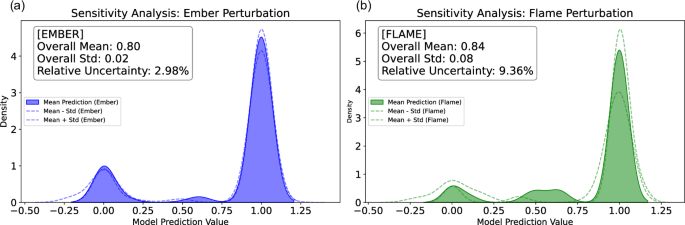
A sensitivity analysis is shown, performed by perturbing two key exposure inputs—ember deposition and flame length—using 100 ensemble outputs from the ELMFIRE spread model (HAMADA extension) for each fire, while holding all other predictors constant. For each test sample (n = 47,742), the model’s predicted survival probability was computed across ensembles to yield a mean prediction (solid fill) and its uncertainty (shaded region = ± 1 standard deviation). a Ember perturbation: blue fill shows the kernel density of mean predictions under varied ember load; dashed blue lines mark mean ± std. Inset reports overall mean, standard deviation and relative uncertainty (%). b Flame perturbation: green fill shows the kernel density of predictions under varied flame length; dashed green lines mark mean ± std. Inset reports overall mean, standard deviation and relative uncertainty (%). This framework quantifies the influence of non-linear interactions and input variability on the binary damage classification (0 = not damaged, 1 = damaged), reveals emergent intermediate prediction modes, and offers both local and global insights into model behavior under uncertainty.
Confusion matrix and ROC curve for predictions
A confusion matrix summarizes the classification performance of a classifier with respect to some test data. It is a two-dimensional matrix, indexed in one dimension by the true class of an object and in the other by the class that the classifier assigns61. Receiver operating characteristics (ROC) graphs are useful for organizing classifiers and visualizing their performance. A receiver operating characteristics (ROC) graph is a technique for visualizing, organizing and selecting classifiers based on their performance62. We investigated the five large WUI fires in our dataset to predict structure survival during each fire by understanding the model’s accuracy, and other key performance metrics. By analyzing the confusion matrices and ROC curves for each fire event, we were able to identify patterns and discrepancies in model performance, leading to a better understanding of the factors influencing structure survival in large WUI fires.
Reporting summary
Further information on research design is available in the Nature Portfolio Reporting Summary linked to this article.