
Research area
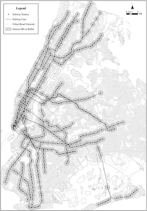
New York City, a global metropolitan hub with significant economic, political, and cultural influence, serves as the research area of this study. It comprises five boroughs: Manhattan, Queens, Brooklyn, the Bronx, and Staten Island. Home to the busiest subway system in the Western Hemisphere, NYC recorded over 3 million daily subway trips in 202436, making it an ideal testbed for research on urban mobility. Its public transportation system, which includes 423 subway station complexes as of the study period (as shown in Fig. 1) and operates 24 hours a day, is the largest and most complex in the United States. Nearly half of NYC residents rely on public transit for their daily commutes, according to the 2022 Citywide Mobility Survey Results, demonstrating a robust dependence during the pandemic period that is unmatched in the U.S.37.
Fig. 1
However, with rising global temperatures, the operation of the NYC subway faces new challenges. According to the U.S. Regional Plan Association38, subway stations are frequently up to 6 °C (10.8 ℉) hotter than above ground. Medical research indicates that even short waiting times in hot, humid, and crowded subway stations can lead to heat-induced health consequences39.
NYC is situated within the humid subtropical climate zone (Köppen Cfa), characterized by hot, humid summers and moderately cold winters (see Fig. 2). These climatic conditions, combined with NYC’s high population density and strong dependence on public transportation, make it a critical case study for exploring the impacts of EHEs on subway ridership and station-level resilience.
Fig. 2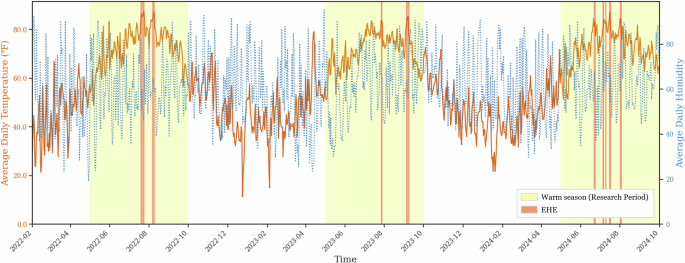
Weather Conditions in NYC from February 2022 to October 2024.
Data preparation and variable definitions
The datasets utilized in this study are categorized into the following types: meteorological data, ridership data, station context data, built environment data, and socio-economic data.
The heat index, derived from the concept of apparent temperature40, estimates how hot it feels when air temperature and humidity are combined. It is calculated using air temperature (T) and relative humidity (RH), following the method developed by Rothfusz41 for the U.S. National Weather Service. Initially, the \({HI}\) is approximated using the following simplified formula:
$${HI}=0.5* T+61.0+\left[\left(T-68.0\right)* 1.2\right]+\left({RH}* 0.094\right)$$
(1)
In practice, this simplified formula is computed first, and the result is averaged with the air temperature. If the calculated heat index exceeds 80 °F, a more complex regression equation, along with any necessary adjustments, should be applied41. The full equation is given as:
$${HI}=-42.379+2.04901523* T+10.14333127* {RH}-0.22475541* T* {RH}-0.00683783* T* T-0.05481717* {RH}* {RH}+0.00122874* T* T* {RH}+0.00085282* T*\, {RH}* {RH}-0.00000199* T* T* {RH} * {RH}-{Adjustment}1+{Adjustment}2$$
(2)
$${Adjustment}1=\left[\left(13-{RH}\right)/4\right]* \sqrt{\left(17-\left|T-95\right|\right)/17}$$
(3)
$${Adjustment}2=\left[\left({RH}-85\right)/10\right]* \left[\left(87-T\right)/5\right]$$
(4)
where \(T\) is the air temperature in degrees Fahrenheit and \({RH}\) is the relative humidity expressed as a percentage. \({HI}\) is the heat index expressed as an apparent temperature in degrees Fahrenheit. \({Adjustment}1\) applies when \({RH}\) is less than 13% and \(T\) is between 80 and 112 °F. \({Adjustment}2\) is valid on the condition that the \({RH}\) is greater than 85% and \(T\) is between 80 and 87 °F. This method provides a more accurate representation of the perceived temperature under conditions of higher heat and humidity.
According to the National Oceanic and Atmospheric Administration (NOAA), when the heat index exceeds 90 °F, prolonged exposure or physical activity can result in heat cramps or heat exhaustion. Environments with a heat index above 125 °F pose extreme danger, with heat stroke becoming highly likely. In this study, we adopt the National Weather Service (NWS) standard to define EHEs based on the criteria for issuing a heat advisory. Specifically, EHEs are defined as periods when the heat index reaches 95–99 °F for at least two consecutive days, or 100–104 °F for any duration. This definition aligns with New York City’s criteria for EHEs42,43. The dates of all identified heat events during the study period are provided in Table S1.
The core ridership data, obtained from MTA, offers subway ridership estimates on an hourly basis, categorized by subway station complex and class of fare payment. The ten consolidated fare payment categories are as follows: “MetroCard – Fair Fare,” “MetroCard – Full Fare,” “MetroCard – Other,” “MetroCard – Senior & Disability,” “MetroCard – Students,” “MetroCard – Unlimited 30-Day,” “MetroCard – Unlimited 7-Day,” “OMNY – Full Fare,” “OMNY – Other,” and “OMNY – Seniors & Disabilities.” From these categories, we can further identify specific passenger groups, such as low-income individuals, seniors, and people with disabilities, who are generally considered socially vulnerable populations.
The NYC Fair Fares program, initiated in January 2020, assists low-income New Yorkers in managing their transportation costs44. Eligible residents can pay half the regular fare for specific transit services, including the subway. Since successful applicants must have an income at or below the federal poverty level (see Table S2), this study identifies passengers using the “MetroCard – Fair Fare” as a low-income group. Additionally, the fare payment classes “MetroCard – Senior & Disability” and “OMNY – Seniors & Disabilities” are combined into the Seniors & Disability group. Daily ridership trends in New York City from 2022 to 2024 are illustrated in Fig. 3.
Fig. 3: MTA Subway Ridership from February 2022 to October 2024.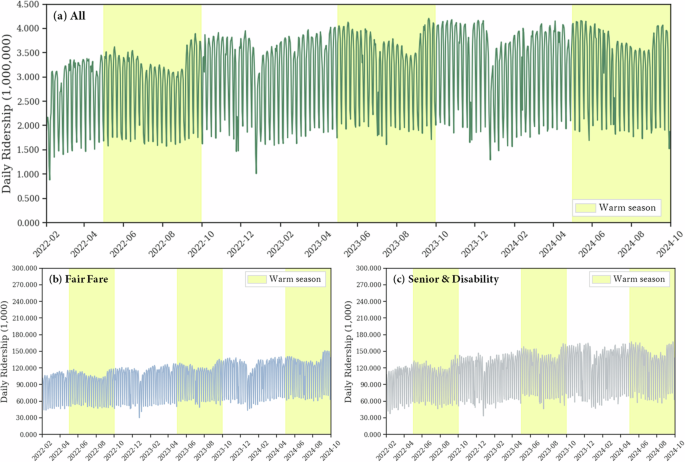
a Total Ridership; b Fair Fares Subgroup; c Seniors and People with Disabilities Subgroup.
The ridership data is used to analyze the temporal and spatial distribution of subway usage on non-EHE days and during EHEs. To minimize the influence of outlier events such as holidays, these days are excluded based on classifications from the Office of Payroll Administration (see Table S3). Additionally, the data is divided into two groups to account for differences between weekdays and weekends.
The distributions of station-level hourly ridership and meteorological conditions (specifically the heat index) during the study period are presented in Figs. S1 and S2. These variables exhibit substantial fluctuations over time. To more accurately capture the relationship between ridership and weather factors, recent research increasingly focuses on the relative change in station ridership, rather than using absolute passenger volumes for regression analysis7,18. The most commonly used approach is the 9-term moving average method45. Following Eqs. (5) and (6), the ridership residuals for different groups are calculated. The detailed distributions are presented in Figs. S3–S5.
$${\bar{r}}_{t}^{{MA}\pm 4}=\frac{{\sum }_{{\rm{\tau }}=-4}^{4}{r}_{t+7{\rm{\tau }}}}{9}$$
(5)
$${e}_{t}=\frac{{r}_{t}-{\bar{r}}_{t}^{{MA}\pm 4}}{{\bar{r}}_{t}^{{MA}\pm 4}}$$
(6)
where \({e}_{t}\) is a daily (or specific time period) ridership residual; \({r}_{t}\) represents either the overall ridership or ridership of specific group during a given day or during a specific time period \({\rm{t}}\); the \({\bar{r}}_{t}^{{MA}\pm 4}\) represents 9-term moving average value for time \({\rm{t}}\); and \({\rm{\tau }}\) represents weeks, with \({\rm{t}}+7{\rm{\tau }}\) ranging from 28 days before to 28 days after, in increments of seven days.
To maintain consistency in passenger distribution and reduce temporal fluctuations, the residuals of meteorological data are calculated using Eq. (7).
$${W}_{\hat{t}}=\frac{{W}_{t}-{\bar{W}}_{t}^{{MA}\pm 4}}{{\bar{W}}_{t}^{{MA}\pm 4}}=\frac{{W}_{t}-\frac{{\sum }_{{\rm{\tau }}=-4}^{4}{W}_{t+7{\rm{\tau }}}}{9}}{\frac{{\sum }_{{\rm{\tau }}=-4}^{4}{W}_{t+7{\rm{\tau }}}}{9}}$$
(7)
where \({W}_{\hat{t}}\) represents the residuals of wind speed, cloud cover, and maximum heat index; \({W}_{t}\) denotes the actual weather values on a given day \({\rm{t}}\); and \({\bar{W}}_{t}^{{MA}\pm 4}\) is the 9-term moving average of the weather values on that day \({\rm{t}}.\) Since most clear days have zero precipitation, the residual precipitation is calculated as the precipitation on that day minus the 9-term moving average.
Finally, to evaluate station-level variation in ridership resilience, we compile a comprehensive set of variables across three domains: station attributes, built environment characteristics, and socio-economic context.
Station attributes include the number of entrances and exits, whether the station is underground, the number of years in operation (as of 2022), and its betweenness centrality within the subway network. Betweenness centrality, calculated using General Transit Feed Specification (GTFS) data, quantifies how often a station appears on the shortest paths between other stations in the transit network and reflects its importance in overall connectivity46.
Built environment characteristics are measured within a 400-meter radius of each station, following the widely used “5 Ds” framework47, which includes density, diversity, design, distance to transit, and destination accessibility. Each of these dimensions plays a crucial role in shaping travel demand. Population density is used to represent urban intensity. To quantify diversity, we include measures of the land use area for different types, as well as an entropy index to represent land use mix. The index reflects the extent to which an area accommodates multiple functions48, where lower entropy values indicate single-use environments. Street network design is captured by calculating the average betweenness centrality of the local road network. Distance to transit and destination accessibility are represented by the number of nearby transit bus lines, bike racks, parking lots, and various types of destinations, including health facilities, commercial centers, and recreational or cultural venues.
Socio-economic context is derived from U.S. Census tract data and aggregated to each station’s surrounding neighborhood using area-weighted averages within the same 400-meter buffer. These indicators include median household income, employment rates, vehicle ownership, and demographic composition, such as the proportions of seniors, women, and minority populations.
Together, these variables provide a multidimensional view of the infrastructural, spatial, and demographic contexts that may influence station-level resilience during EHEs. Detailed definitions, data sources, and descriptive statistics for all variables are presented in Table 1.
Table 1 Variable Definitions and Descriptive StatisticsModeling approach
After deriving the variables and conducting Variance Inflation Factor tests (see results in Table S4), we first employ multivariate linear regression to analyze the impact of EHEs on ridership fluctuations, controlling for other weather factors as well as year and month fixed effects.
$${e}_{t}={\beta }_{0}+{\beta }_{1}{EHE}+{\beta }_{2}{W}_{t}+{\beta }_{3}{W}_{\hat{t}}+\gamma {YearFixed}+\delta {MonthFixed}+\varepsilon$$
(8)
where \({e}_{t}\) represents the station ridership residual on day \(t\); \({EHE}\) denotes whether the day falls within an EHE event; \({W}_{t}\) and \({W}_{\hat{t}}\) represent the observed meteorological conditions and their residuals for day \(t\), respectively; \({YearFixed}\) and \({MonthFixed}\) correspond to the year and month fixed effects; \({\beta }_{0}\) is the model intercept; \({\beta }_{1}\),\({\beta }_{2}\), \({\beta }_{3}\), \(\gamma\) and \(\delta\) are parameters for estimation; and \(\varepsilon\) is the error term.
Subsequently, we conduct a Welch’s t-test, a two-sample t-test that does not assume equal variances, to assess whether ridership residuals at each station during EHEs differ significantly from those during non-EHE periods. This method accounts for potential differences in sample size and variance between comparison groups. We employ a 10% significance level (p < 0.10) to balance the risks of Type I and Type II errors in this exploratory residual-based analysis. To control for false discoveries from multiple station-level comparisons, we apply the Benjamini-Hochberg procedure, which maintains the expected false discovery rate at or below 10%. The results of this analysis are presented in Fig. S6. The use of a 10% significance level is consistent with established practices in transportation research involving exploratory spatial data analysis, ridership determinants, and assessments of climate impacts on travel behavior49,50,51. Importantly, our analysis is based on residuals derived from ridership models that adjust for temporal trends, seasonal variation, and baseline station characteristics, rather than raw ridership counts. This residual-based approach reduces unexplained variance and enhances the sensitivity of the test to EHE-specific effects, thus justifying a moderately relaxed significance threshold. Given the exploratory nature of this station-level analysis, the consequences of Type II errors (i.e., failing to detect genuinely affected stations) may outweigh those of Type I errors. Missing vulnerable stations could hinder evidence-based transit adaptation strategies in response to climate risks. To further mitigate error inflation due to multiple testing, the Benjamini-Hochberg correction ensures that the expected proportion of false discoveries among statistically significant findings remains at or below 10%, independent of the nominal alpha level.
Based on these test results, stations are classified into three categories: those exhibiting a significant decline in ridership during EHEs, those showing an increase, and those experiencing negligible fluctuations. Following the concept introduced by Li et al.52, we reclassify stations with reduced ridership as low resilience, while the other two categories are designated as high resilience.
Finally, we employ a probit model to examine the relationship between station attributes, the built environment, and the socioeconomic context in relation to ridership resilience levels.
$${Y}^{* }=\alpha X+\tau$$
(9)
where \({Y}^{* }\) is the latent dependent variable, X denotes the independent variables, and \(\tau\) is the error term. The predicted binary variables for cluster Y = 1 if Y* ≥ 0, Y = 0 otherwise.