

Data generation and neural network training
To develop a neural network potential with DFT accuracy in energy and forces for few-layer TMD and moiré superlattices, we adopt a systematic “active learning” approach to generating our DFT dataset. We train the potential with small unit cells, in contrast to using twisted bilayer TMDs, minimizing the cost associated with DFT calculations. A schematic representation of the active learning workflow is shown in Fig. 1. We start with monolayer, homobilayer, and strained TMD bilayer heterostructures. For proper sampling of the potential energy surface of layered TMDs, we consider polymorphs with both AA and AB stacking, forming a total of 35 structures (i.e., 5 monolayers, 5 homobilayers, each of AA and AB stacking; and 10 AA and AB heterostructures each). Behler-Parrinello symmetry function-based neural network potentials (NNPs) are employed in the active learning loop. Due to the van der Waals interlayer interactions in TMDs, we incorporate a model van der Waals r−6 form following the work presented in ref. 49, as described below. Initially, we train an ensemble of neural network potentials on a dataset constructed from random displacements of atomic coordinates of monolayer unit cells and AB-stacked bilayers TMDs. For each system, we generate 500 configurations. The displacements relative to equilibrium in each case are drawn from a Gaussian distribution with a fixed Gaussian width of 0.05 Å. In this work, we use an ensemble of NNPs with a size of 5. One of the NNPs is used to run molecular dynamics (MD) simulations at multiple temperatures and pressures for each system, including the AA stacked bilayer TMDs for 200,000 time steps. Each time step corresponds to 1.0 fs. To minimize the finite size effects, we use 3 × 3 × 1 supercells, which gives rise to simulation cells containing 27 atoms and 54 atoms for monolayers and bilayers, respectively.
Fig. 1: Workflow describing data generation and neural network training.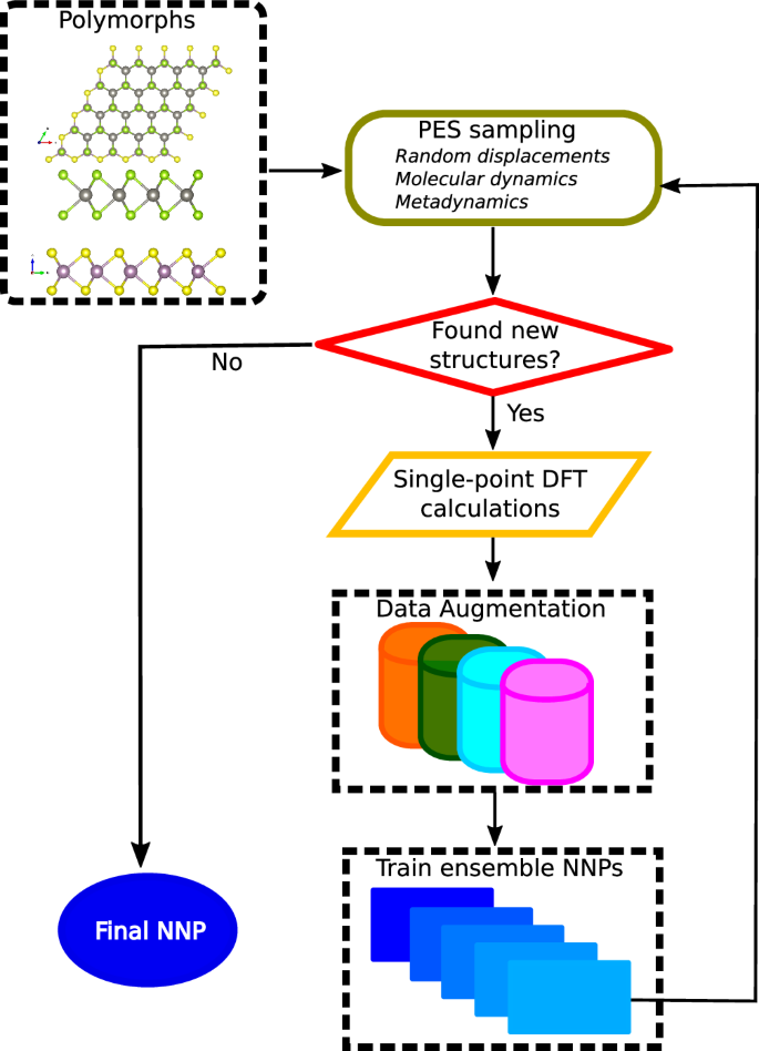
Starting from polymorphs containing monolayers and bilayer TMDs, we perform the potential energy surface (PES) sampling through random displacements (at the initial steps), molecular dynamics simulations, and metadynamics at finite temperatures and pressures, followed by check for new configurations, single point DFT calculations, data augmentation, and NNP trainings. The workflow is detailed in the main text.
Our MD simulations are performed at pressures of 0 and ±1 GPa and at temperatures of 300 and 800 K. For each pair of pressure and temperatures, we collect snapshots from our trajectories every 200 time steps, giving rise to 1000 configurations per structure. In order to minimize the number of DFT calculations and to reduce redundancy and bias in our sampling during our active learning loop, we compute the ensemble root-mean-square deviation on each snapshots based on their energies using the five trained NNPs. Only snapshots whose ensemble error is above 2.5 meV/atoms are computed with DFT and added to the previously generated training dataset. This procedure is repeated until there are no new snapshots with large ensemble errors found via the unbiased molecular dynamics simulations.
In order to sample environments different from strictly AA and AB stacking, which are not easily accessible in an unbiased MD at the temperatures considered here, we employ metadynamics simulations with collective variables corresponding to the interlayer distances between the nearest neighbor transition metals from different TMD monolayers. In this way, the potential energy surface associated with the sliding of one layer relative to the other is efficiently sampled. Additionally, this approach avoids large unit cells of twisted bilayer TMDs, as all the chemical environments present in twisted TMDs can be sampled. Our metadynamics calculations are performed at 300 K.
From the active learning cycle and metadynamics simulations, a total of ~89,400 configurations are generated. Finally, to capture interactions between the TMD and a boron nitride substrate in our NNP model, we added TMD-hexagonal boron nitride (hBN) configurations in two steps. First, we generate 100 randomly displaced configurations for each of the five monolayer TMDs supported on a single-layer hBN, as well as 100 configurations of single-layer hBN and retrain the NNP model; second, we use the trained model to generate additional data from MD simulations at 300 K. We then extract snapshots at regular intervals and then perform a single-point DFT calculations. The total number of structures in the dataset is ~92,600. 90% of the dataset prior to adding hBN data, and the entire dataset with hBN configurations are used for training, while the remaining 10% is used to test the model.
Neural network potential
We construct our neural network potentials using modified Behler-Parrinello symmetry functions (BPSFs)34,35 to describe the chemical environments as implemented in the PANNA software36,50. We chose cutoffs of 8 Å and 4 Å for the radial, which encode two-body information, and angular descriptors, that describe three-body atomic interactions, respectively. We sample the radial centers in the radial descriptors with 43 uniformly-spaced Gaussians starting at 0.5 Å with a fixed Gaussian width of 33 Å−2. This gives rise to a 7 × 43 = 301 vector size for a seven-species system. For the angular part, we use 16 evenly spaced angular centers with no angular radial sampling. In this case, the angular component of the descriptors has dimensions \(\frac{7\times 8}{2}\times 16=448\) for the seven-species system. The radial and the angular descriptors are then concatenated to form the input vectors of the fully connected feed-forward neural network, giving rise to an input vector dimension of 301 + 448 = 749. We use a neural network architecture with two hidden layers of 64 nodes each and a single node output layer that corresponds to the atomic energy of each atom.
To account for van der Waals interactions, we add an energy term to the standard Behler–Parrinello neural network potential following the expression proposed in ref. 49. This term takes the general form
$${E}_{vdw}=-\frac{1}{2}\sum _{ij}{C}_{6ij}\frac{{S}_{up}({x}_{ij}){S}_{down}({x}_{ij})}{{r}_{ij}^{6}},$$
(1)
where
$${S}_{down}(x)=\left\{\begin{array}{ll}1,\quad &{\rm{if}}\,x < 0\\ -6{x}^{5}+15{x}^{4}-10{x}^{3}+1,\quad & {\rm{if}}\,0\le x\le 1\\ 0,\quad &{\rm{otherwise}}\end{array}\right.$$
are functions that allow a smooth transition to long-range interactions at a user-specified cutoff, and \({x}_{ij}=\frac{{r}_{ij}-{r}_{min}}{{r}_{max}-{r}_{min}}\); Sup(x) = 1 − Sdown(x) controls the contribution of the van der Waals energy term in the short-range, where the local environment-based model is active.
In ref. 49, C6ij was taken as a constant denoted as A, and was obtained from a fit to the interlayer binding energy of bilayer graphene. For multispecies systems such as TMDs, using a constant parameter for the C6 coefficient is inadequate. Instead, here we let the coefficient depend on the type of atom i and j. We further decompose C6ij as a geometric sum of the atomic C6 coefficients, \({C}_{6ij}=\sqrt{{C}_{6i}{C}_{6j}}\), similar to what is commonly done in the Grimme D-type van der Waals correction51. The atomic C6 coefficients are obtained from ref. 52. In this work, we include van der Waals interactions up to rmax = 12 Å, and chose rmin = 11 Å as the onset of the decay to zero at rmax. At short distances, the van der Waals contribution goes to zero smoothly at \({r}_{\min }=6\) Å with the damping starting at \({r}_{\max }=8\) Å. It is worthwhile to note that the van der Waals functional form proposed here can be readily incorporated into state-of-the-art equivariant NNPs frameworks.
Training and validation
In this section, we discuss the accuracy of our model as obtained via the approach outlined in “Results”. The neural network potentials are trained using the Adam optimizer53, a stochastic gradient decent optimization algorithm, with a batch size of 16 and an initial learning rate of 0.001 that exponentially decays at a rate of 1% for every 5000 training steps. The mean absolute error (MAE) on energy and forces on the training set is 0.75 meV/atom and 14.52 meV/Å, respectively. For the test set, we obtain an MAE of 0.74 meV/atom in energy and 14.33 meV/Å in forces. The training and test MAE are similar, implying that there is no overfitting on unseen configurations.
The energy correlation between DFT and our NNP resolved with respect to the subsystem in the training dataset is shown in the Supplementary Figure 1. We find excellent agreement between DFT and NNP energies across the subsystems, reflecting the small mean absolute error in energy of 0.74 meV/atom in the test set and indicating transferability of the final NNP. Similar agreement between DFT and our NNP is observed in the atomic forces (see Supplementary Fig. 2).
Interlayer binding and sliding energetics
In this section, we describe the extensive testing of our potentials on the TMD interlayer binding energy as a function of (i) the interlayer separation, defined as the distance between the transition metals along the perpendicular direction, denoted as dM; and (ii) the sliding distance that probes the stacking dependence of the binding energy at a fixed interlayer separation. It has been demonstrated that an interatomic potential that accurately captures the interlayer binding energy along these coordinates (interlayer spacing, dM, and sliding distance, here denoted by δ) is suitable for obtaining accurate ground-state relaxed structures of moiré superlattices33 because all chemical environments found in TMD moiré superlattices can be sampled. The binding energy, ΔE, associated with a bilayer TMD is defined as
$$\Delta E=\frac{E({\rm{bilayer}})-E({\rm{monolayer}}1)-E({\rm{monolayer}}2)}{N},$$
(2)
where E(bilayer) is the total energy of the bilayer with N atoms, E(monolayer1) is the total energy of the first monolayer, and E(monolayer2) is the total energy of the second monolayer.
In Fig. 2, we show the example of WS2/MoSe2 bilayer, illustrating different realizable stacking configurations starting from AA stacking (Fig. 2a–c) and AB stacking (Fig. 2d–f).
Fig. 2: Bilayer TMD high-symmetry structures.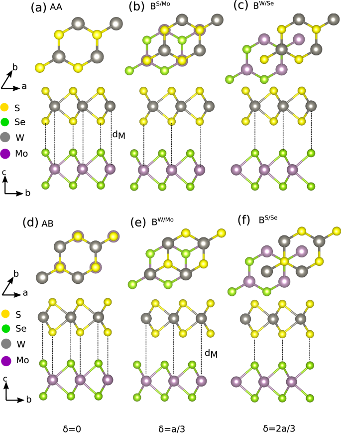
High-symmetry structures at different sliding distances, δ, for bilayer TMDs, starting from the AA and AB stacking configurations. a AA stacking with W on Mo and S on Se at δ = 0; b Bernal stacking with S on Mo at \(\delta =\frac{1}{3}a\); c Bernal stacking with W on Mo at \(\delta =\frac{2}{3}a\); d AB stacking with W on Se at δ = 0; e Bernal stacking with W on Mo at \(\delta =\frac{1}{3}a\); and f Bernal stacking with S on Se at \(\delta =\frac{2}{3}a\).
Here, we start with homobilayers and focus on systems containing Mo; W-containing systems follow the same trends and are discussed in the Supplementary Fig. 3. In Fig. 2, we illustrate the geometry of WS2/MoSe2 bilayers. Figure 3a, c, e show the binding energies of MoS2, MoSe2, and MoTe2 homobilayers as function of interlayer spacing, dM, comparing our NNP model with DFT results. We also depict the composition of the two interacting layers at the right-hand side of each plot. Our NNP reproduces the DFT binding energy accurately, even at large dM, for both AA and AB stacking. To quantify the accuracy of our NNP potential energy surface as a function of sliding, we generate configurations for AA and AB stacking by sliding one layer relative to the other at a fixed interlayer spacing. The interlayer spacing for both AA and AB stacking is fixed at the AB stacking equilibrium interlayer spacing for each structure. These interlayer spacings can be read from Fig. 3a, c, e. In Fig. 3b, d, f, we show the interlayer binding energy for MoS2, MoSe2, and MoTe2 homobilayers. Overall, all features of the DFT potential energy surface are well captured by our NNP, namely: the minima at δ = 0 and δ = a/3 for AB stacking (see Fig. 2d, e, f) and the minima at δ = a/3 and δ = 2a/3 for AA stacking (see Fig. 2a, b, c). These results demonstrate that our NNP can be used to simulate the properties of TMD homobilayers at near-DFT accuracy.
Fig. 3: Interlayer binding energy of homobilayer TMD.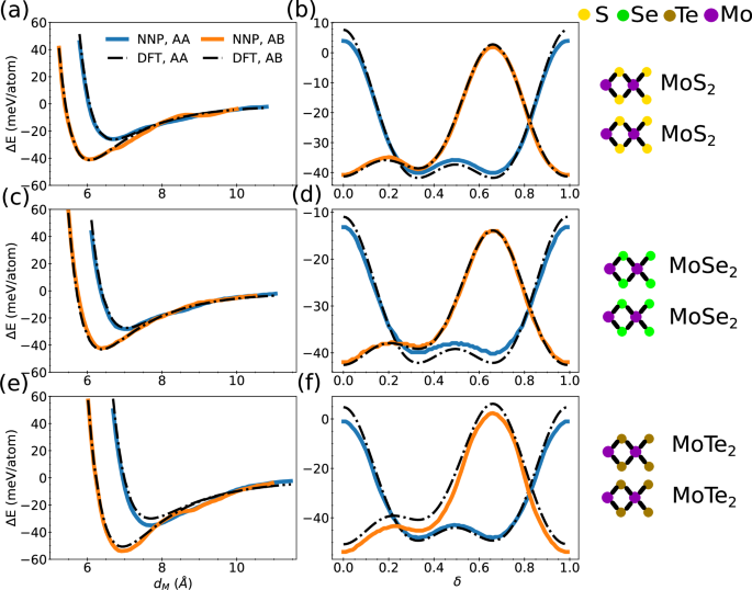
Interlayer binding energy, ΔE, for TMD homobilayers as a function of interlayer distance, dM, for a MoS2, c MoSe2, and e MoTe2, and as a function of sliding distance, δ, for b MoS2, d MoSe2, and f MoTe2. Here, δ is given in units of the in-plane lattice spacing.
Next, we discuss the accuracy of our model for the potential energy surface of TMD bilayer heterostructures. In Fig. 4, we show the interlayer binding energy of TMD heterostructures as a function dM and δ for MoS2/MoSe2, MoS2/MoTe2, and MoSe2/MoTe2 systems. In the case of the binding energy with respect to dM, the NNP model captures the DFT potential energy surface accurately for all systems. Similarly, our van der Waals-corrected NNP is in good agreement with the DFT potential energy surface along the sliding distance, δ, for all the heterostructures considered here.
Fig. 4: Interlayer binding energy of bilayer TMD heterostructure.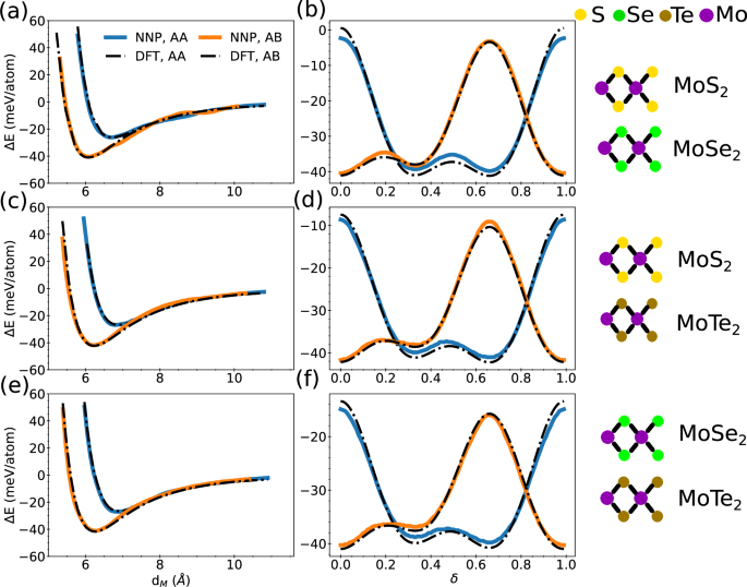
Interlayer binding energy, ΔE, for TMD heterostructures as a function of interlayer distance, dM, for a MoS2/MoSe2, c MoS2/MoTe2, and e MoSe2/MoTe2, and as a function of sliding distance, δ, for b MoS2/MoSe2, d MoS2/MoTe2, and f MoSe2/MoTe2.
Vibrational properties
In this section, we discuss the vibrational properties of homobilayer TMDs to assess the applicability of our NNP model in describing the dynamical properties of layered TMDs. Accurate prediction of vibrational properties is required for the study of thermal transport with lattice dynamics approaches that consider phonon scattering. Vibrational frequencies are usually challenging to accurately predict using empirical force fields because they are fit, at most, to only the acoustic branch of the phonon dispersion32, making them unreliable for other phonon branches in the Brillouin zone (BZ). We have previously shown that NNPs trained on energy and forces can accurately predict DFT phonon spectra across the entire BZ for carbon systems40 and for amine-appended metal-organic frameworks42. Here, we focus on Mo-containing bilayer systems, and the results obtained for monolayer Mo systems and all W-containing systems are shown in the Supplementary Fig. 4. All systems are fully relaxed before computing the vibrational frequencies. We use finite difference methods as implemented in phonopy54, with uniform atomic displacements of 0.015 Å and forces as input, to construct the dynamical matrix from which the phonon frequencies and eigenvectors are computed. For our NNP, we evaluate the atomic forces for each displaced configuration using the LAMMPS package55.
In Fig. 5, we compare the phonon dispersion in monolayer MoS2 obtained with the Stillinger-Weber potentials and our NNP with DFT and experiments. The phonon dispersion is computed along the direction connecting hexagonal high symmetry points, Γ(0,0,0), M (1/2,0,0), and K (2/3,1/3,0). Our NNP results are in excellent agreement with both DFT and experiments56. However, results with Stillinger–Weber potential deviate significantly from both DFT and experimental results, limiting their ability to reliably predict the transport properties in TMDs because of their crude depiction of vibrational modes relevant to thermal transport57.
Fig. 5: Phonon dispersion of monolayer MoS2.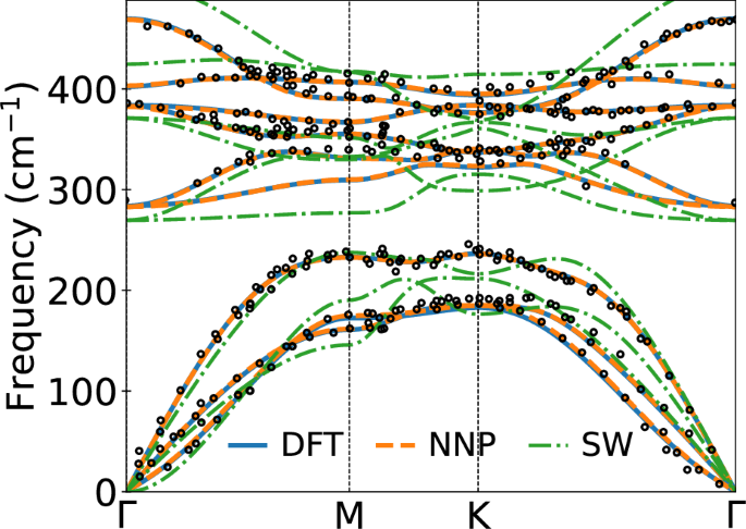
Computed phonon dispersion of MoS2 monolayer with SW potential, our NNP, and DFT. The black open circles are experimental data obtained from ref. 56.
Figure 6a, b, c depict the phonon band structure of bilayer MoS2, MoSe2, and MoTe2, respectively. For all three phonon band structures, our NNP captures the DFT vibrational frequencies exceedingly well, further confirming the transferability of our NNP to quantities that depend on the second derivative of the total energy. More interestingly, both the DFT and NNP results agree well with the experimental data, signifying that (i) vdW-DF-C09 can accurately reproduce the experimental data and (ii) the trained NNP can readily replace DFT in the computation of vibrational properties of layered TMDs.
Fig. 6: Phonon dispersion of bilayer MoS2.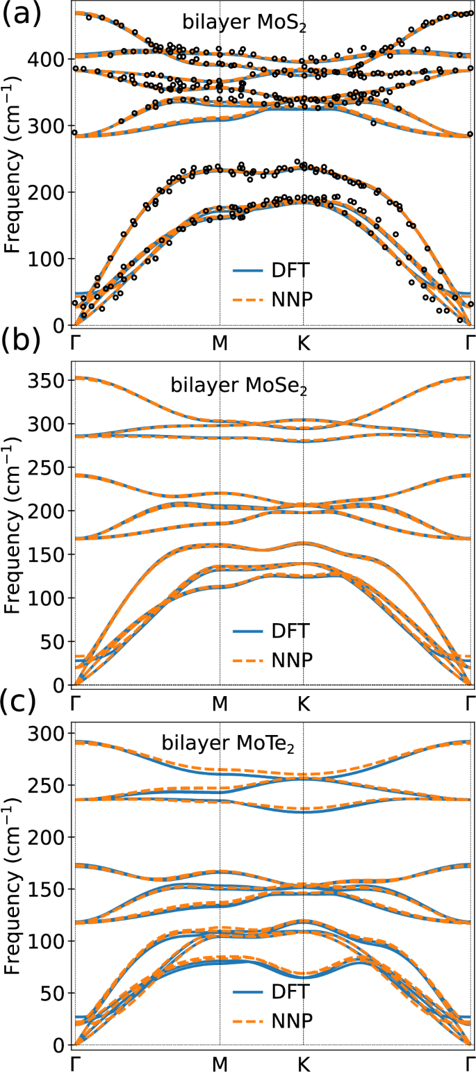
Computed phonon dispersion of Mo-containing homobilayer systems. a MoS2, including results from experiments56 (black open circles) b MoSe2 and c MoTe2.
Atomic forces in large-angle moiré superlattices: invariant versus equivariant models
After we demonstrate the accuracy of our NNP for both homobilayers and heterostructures, we now turn to moiré superlattices. The accuracy of the NNP for atomic forces of large-angle moiré superlattices is expected to be a good indication of its transferability and applicability to larger moiré structures, especially atomic reconstructions of small-angle twisted bilayer TMDs and heterostructures. To quantify the accuracy of our van der Waals-corrected NNP on moiré superlattices, we perform single-point calculations on twisted MoS2, MoSe2, MoTe2, MoS2/MoSe2, and MoS2/MoTe2 bilayers and compare with the DFT predicted forces. To limit the number of atoms, all test systems are twisted at an angle of 9.4° and 50.6°. We construct twisted bilayer TMDs following the approach described in ref. 58. For twisted homobilayers, we obtain moiré superlattices with 222 atoms; for heterostructures, we generate moiré lattices with a strain below 5 %, giving rise to 222 atoms for MoS2/MoSe2 and 420 atoms for MoS2/MoTe2. The interlayer distances are fixed at the DFT AB values of 6.04, 6.38, and 6.91 Å for MoS2, MoSes, and MoTe2, respectively. For the heterostructures, we use the average AB interlayer spacing of the homobilayers.
In order to assess the importance of van der Waals corrections, we compare our van der Waals corrected NNP with the standard PANNA model and MACE44, a state-of-the-art machine learning architecture that combines equivariant message passing neural network methods with many-body messages via a body-order energy expansion. A foundation model59 based on the MACE architecture was recently trained on the Materials Project database60, which primarily contains bulk systems. In this work, we train the MACE model on a specialized dataset of TMD layers, generated here, to enable a proper comparison with our van der Waals-corrected NNP. All models are trained with a maximum cutoff of 8 Å. The three-body interactions in PANNA are treated up to 4 Å; MACE applies a cutoff of 8 Å for the two-, three-, and four-body interactions. In this work, we use two-body atomic feature mixing channels of 128; correlation order of 3, corresponding to two-to-four-body interactions; and equivariant symmetry order of L = 0.
Furthermore, we evaluate the effects of fixed atomic C6 coefficients. To this end, we modify the atomic C6 coefficient to depend on the chemical environment such that \({{\rm{C}}}_{6}={{\rm{C}}}_{6}\times (1+\frac{{\rm{dC}}}{2})\). The environment-dependent quantity, dC6, is predicted as the second component of the output layer of the atomic neural network that returns two numbers, the first one representing the atomic energy. The predicted dC6 is constrained to take values between −1 and 1 through a hyperbolic tangent activation function. The final C6 parameters are only allowed to changed by at most 50 %. Here, we compare the layer binding energy as well as the atomic forces on twisted bilayer TMDs.
The accuracy of these models is compared using the mean absolute energy and force as metrics on out-of-sample large-angle twisted bilayer TMDs. In Fig. 7 we show the mean absolute error in the total energy obtained with the van der Waals corrected NNP with and without learnable atomic C6 coefficients. For the systems containing MoS2 and MoSe2, including heterostructures, our NNP with van der Waals corrections performs as well as the MACE model and our NNP without dispersion correction. However, systems that include MoTe2 are more challenging for both MACE and our NNP without dispersion. In Fig. 8, we compare the NNP forces on the moiré superlattices with those from DFT. The inset shows bar plots of the mean absolute errors with respect to DFT. The errors are mostly below 25 meV/Å for dispersion aware models and MACE for both on homobilayer and heterostructures, except for Te containing systems where our short-range model (without dispersion) has a much larger mean absolute error.
Fig. 7: NNP prediction error in energy for twisted bilayer TMDs.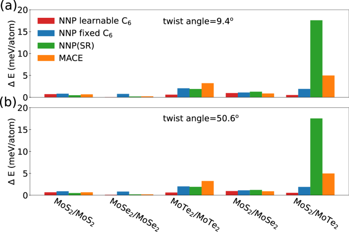
Summary of prediction of NNPs for the twisted bilayer TMDs energies computed with a fixed interlayer spacing at twist angles of a 9.4° and b 50.6°.
Fig. 8: NNP prediction error in forces for twisted bilayer TMDs.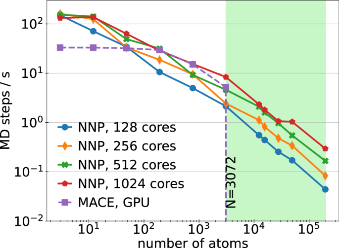
Comparing the computational cost of our NNP with the MACE model. Our model is implemented on CPU while MACE isoptimized for GPU. The green shaded area represent the number of atoms above which our trained MACE model fails due to outof-memory error.
While our NNP with van der Waals corrections outperforms the MACE model for prediction of energies in the out-of-sample dataset, the MACE model is slightly better in predicting forces in some cases. The overall accuracy of our dispersion-aware model is a confirmation that our NNP trained on carefully constructed unit cells is transferable to moiré superlattices. It is important to note that the current implementation of MACE is primarily limited to smaller systems, whereas our dispersion-corrected NNP can simulate systems with over a hundred thousand atoms. We quantify the efficiency of our NNP model by estimating the number of MD steps per seconds obtained from a 100 steps molecular dynamics simulation under microcanonical ensemble (NVE) as a function of the number of atoms (See Fig. 9). Our results show that the MACE model is not scalable to TMD systems with over 3000 atoms while our NNP scales to a hundred of thousand of atoms. The performance can be improved through multi-CPU and multi-compute node supercomputers, a clear advantage over MACE models that are only currently optimized for a single GPU. This makes our approach more efficient for this class of materials and suitable for further analysis.
Fig. 9: Computational cost of NNP.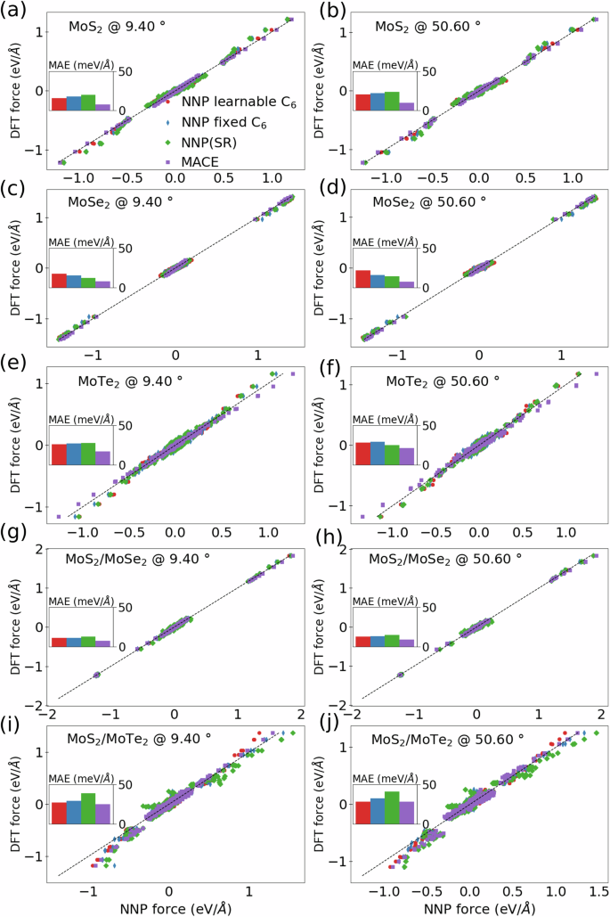
Correlation plot between NNPs and DFT forces for twisted homobilayer and heterostructures: a MoS2 at 9.4°, b MoS2 at 50.6°, c MoSe2 at 9.4°, d MoSe2 at 50.6°, e MoTe2 at 9.4°, f MoTe2 at 50.6°, g MoS2/MoSe2 at 9.4°, h MoS2/MoSe2 at 50.6°, i MoS2/MoTe2 at 9.4°, and j MoS2/MoTe2 at 50.6°.
WS2 twisted bilayers
Here, we test the application of our NNP on twisted bilayers where experimental results are available. We start by using the NNP to predict the interlayer spacing and the relative energy of the high symmetry stacking of bilayer WS2 at zero twist angle, namely, the AA, AB, and Bernal stacking. Our NNP predicted interlayer spacing for AA, AB, and Bernal stacking are 6.730 Å, 6.165 Å, and 6.133 Å, respectively. These are in good agreement with the DFT predicted values of 6.704 Å, 6.194 Å, and 6.127 Å for AA, AB, and Bernal stacking, respectively. Similarly, our NNP predicted energies of AA and Bernal stacking relative to the AB stacking are −15.14 and −3.31 meV/atom, respectively, in excellent agreement with the values of −14.59 and −4.02 meV/atom obtained with DFT.
Next, we generate WS2 twisted bilayers with twist angles of 57.550°, 57.719°, 57.995°, and 51.110° in accordance with the experiment sample, which features a near 58° twist angle. This enables us to investigate the dependence of the atomic relaxation on the twist angle while also validating the accuracy of our NNP against experimental measurements of atomic relaxations.
We use a DFT-optimized lattice parameter of 3.146 Å and start at the AB interlayer spacing of 6.13 Å. We check that the final relaxed twisted bilayer WS2 is robust against the starting interlayer spacing. The total energy of the moiré superlattice is minimized until the atomic forces are below 10−3 eV/Å.
In Fig. 10a–d, we show a heat map of the corrugations of WS2 twisted bilayers. We see a maximum corrugation height increases from 27 p.m. to 32 p.m. at Bernal stacking, denoted as BS/S, indicating the S atoms in the top layer sit directly on an S atom in the bottom layer WS2. This is in agreement with the measured scanning-tunneling microscopy (STM) corrugation profile height of 32 p.m.24. The lowest corrugation height is around the high symmetry stacking, AB (W atom on S atom and vice-versa), followed by Bernal stacking denoted as BW/W (W atoms on the top layer directly on W atom). The difference between the corrugation height for AB and BW/W stacking is small owing to their similar interlayer spacing, which is ~0.06 Å as predicted by vdW-DF-C09 functional.
Fig. 10: Atomic relaxations in twisted WS2 bilayers.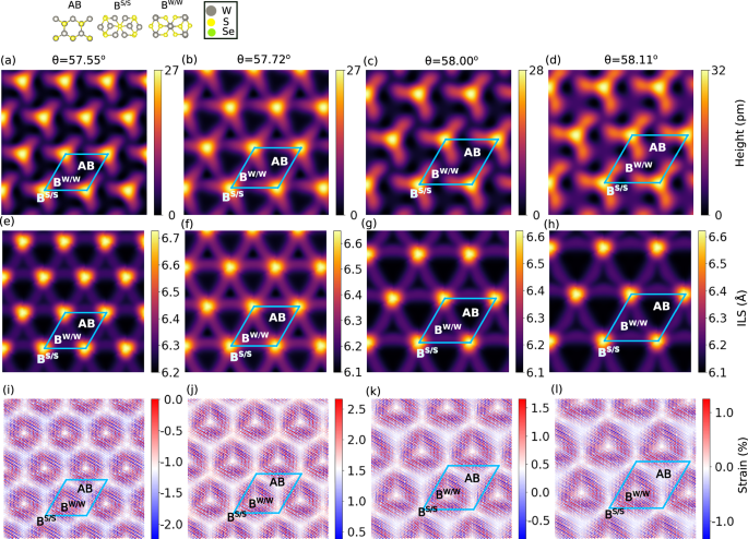
a–d atomic corrugations of the top layer at twist angles, θ, of 57.550°, 57.719°, 57.995°, and 51.110°, e–h the interlayer spacing (ILS) measured as the distance along the z-axis between W atoms; and i–l the strain of W-W bond with respect to the equilibrium lattice parameters.
We also compute the interlayer spacing between W atoms in the two layers (see Fig. 11b) and the local W-W strain (computed with respect to the lattice parameters of monolayer WS2 of 3.146 Å)(see Fig. 11c) in the WS2 twisted moiré superlattice. The maximum interlayer spacing is observed at BS/S, which is 6.65 Å, and the minimum at the AB stacking spacing of 6.13 Å. For W-W local strain, we find close to zero strain in the high symmetry stacking regions. The finite strains occur around the transition between the high symmetry points, which corresponds to high energy regions of the moiré superlattice.
Fig. 11: Atomic relaxation of in MoS2/WSe2 heterostructures at zero twist angle.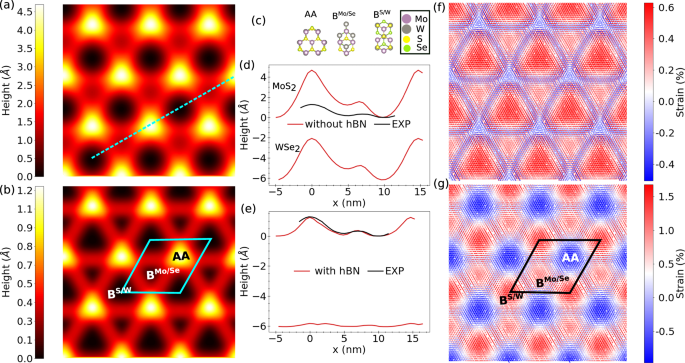
Atomic relaxation of in MoS2/WSe2 heterostructures at zero twist angle. Heatmap depiction of the corrugation of the MoS2 layer showing high symmetry region in the moiré superlattice a free standing TMD b TMD supported on hBN substrate. c High-symmetry stacking arrangements in MoS2/WSe2 heterostructures. Height profile along the line cut shown in a for d free standing TMD and e the TMD supported on a hBN substrate. Local Mo–Mo strain distribution f without and g with hBN substrate.
We note a variation in the corrugations, interlayer spacing, and local strain distribution going from a twist angle of 57.550° to 51.110°. This sensitivity to the twist angle may lead to different electronic structures, a topic of future study.
From these results, we see that the NNP developed here can accurately capture atomic-scale moiré superlattice reconstruction and therefore can be employed to simulate and understand the nature of atomic reconstruction in moiré superlattices.
MoS2/WSe2 heterostructure on hBN
Bilayer TMD heterostructures corrugate due to atomic-scale reconstruction that minimizes in-plane atomic strain originating with the lattice mismatch between the two TMDs monolayers. Here, we investigate the atomic reconstruction and the effects of an hBN substrate on the corrugation of MoS2/WSe2 heterostructures. Our MoS2/WSe2 heterostructure is generated with a fixed interlayer distance of 6.21 Å, corresponding to the average DFT interlayer spacing of 6.04 Å and 6.38 Å for MoS2 and WSe2, respectively. We used the DFT-optimized in-plane lattice parameters of 3.146 Å and 3.266 Å for MoS2 and WSe2, respectively. The lattice mismatch is below 0.1%. Experimentally, bilayer TMDs are often on a substrate, frequently few-layer hBN or epitaxial graphene, providing a mechanical support. The substrate is expected to reduce the TMD out-of-plane degrees-of-freedom and minimize the corrugation heights of the TMD layers. Here, we perform calculations of TMD supported on clamped single-layer hBN. For a free-standing MoS2/WSe2 bilayer, the number of atoms per simulation cell is 4215, and in the presence of hBN layer, there are 6527 atoms. An additional strain of 0.2% is incurred upon adding the hBN substrate. All configurations are relaxed until atomic forces are below 10−3 eV/Å.
In Fig. 11, we show the NNP-predicted corrugation height of the MoS2/WSe2 heterostructures with and without a hBN substrate. In the absence of the hBN substrate (see Fig. 11a, b), the predicted corrugation profile accurately maps out the three high symmetry stackings, namely, AA (Mo atoms on W atoms and S atoms on Se), BS/WMo/Se (Mo atoms on Se) and BS/WS/W (S atoms on W) and agrees well with experimental results61, although the corrugation height profile is overestimated. However, when the bilayer TMD is supported on hBN, we observe excellent agreement between experiment and NNP results (see Fig. 11d, e), underscoring the role of substrate in corrugations of bilayer TMD heterostructures. As expected, the hBN substrate provides a mechanical boundary condition and acts to clamp the TMD layer, consequently lowers the corrugation of the topmost layer.
Furthermore, we can analyze the effect of the hBN substrate on the Mo-Mo local strain redistribution. We compute local strain with respect to the optimized lattice parameter, a0, of the primitive unit cell of MoS2, where we define strain = (dMo−Mo − a0)/a0 * 100. Positive strain corresponds to a local tensile expansion, and negative values of the strain corresponds to a local compression. Figure 11c, f shows the local strain computed in this way. We observe a local compression in the AA stacking region and an expansion in the Bernal stacking regions, BS/WMo/Se and BS/W. The strain at BS/WMo/Se is higher than that at BS/WS/W. These results are in good agreement with experiments61. The observed trend in the local strain is the same with or without the hBN substrate. However, the magnitude of the strain is larger in the TMD heterostructure when supported on an hBN substrate. The increase in the local strain can be attributed to the constraint imposed on the TMD by the clamped hBN substrate that prevents further strain minimization.