Optical generative models | Nature

Snapshot optical image generation process

The snapshot optical generation procedure includes two parts: the digital encoder and the optical generative model. For image generation of MNIST, Fashion-MNIST, Butterflies-100 and Celeb-A, the digital encoder architecture that we selected is a variant of the multi-layer perceptron54, which contained Ld fully connected layers, each of which was followed by a subsequent activation function κ. For a randomly sampled input \({\mathcal{I}}(x,y) \sim {\mathcal{N}}({\bf{0}},\,{\bf{I}})\), where \(x\in [1,\,h],y\in [1,w]\) with h and w denoting the height and width of the input noise pattern, respectively, the digital encoder processes it and outputs the encoded signal \({{\mathcal{H}}}^{({l}_{d})}\) with a predicted scaling factor s (refer to Supplementary Information section 1.1 for details). The one-dimensional output signal of the digital encoder is reshaped into a 2D signal \({{\mathcal{H}}}^{({L}_{d})}\in {{\mathbb{R}}}^{h\times w}\). For the Van Gogh-style artwork generation, the digital encoder consists of three parts: a noise feature processor, an in silico field propagator and acomplex field converter (refer to Supplementary Information section 1.2 for details). The random sampled input is processed to a 2D output signal \({{\mathcal{H}}}^{({l}_{d})}\in {{\mathbb{R}}}^{h\times w}\) and is forwarded to the subsequent optical generative model as outlined below.

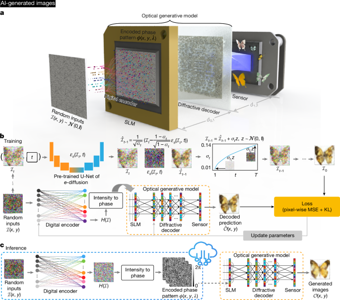
In our implementation, the optical generative model, without loss of generality, consisted of an SLM and a diffractive decoder, which included Lo decoding layers. To construct the encoded phase pattern \(\phi (x,{y})\) projected by the SLM, the 2D real \({{\mathcal{H}}}^{({L}_{d})}\) was normalized to the range \([0,\alpha {\rm{\pi }}]\), which can be formulated as:

$$\phi (x,\,y)=(\alpha {\rm{\pi }}({{\mathcal{H}}}^{({L}_{d})}+1))/2$$

(1)

Here, α is the coefficient controlling the phase dynamic range.

After constructing the incident complex optical field profile \({{\mathcal{U}}}^{(0)}(x,y)=\cos (\phi (x,y))+i\sin (\phi (x,y))\) from the encoded phase pattern, the light propagation through air was modelled by the angular spectrum method55, where \(i\) is the imaginary unit. The free-space propagation of the incident complex field \({\mathcal{U}}(x,y)\) over an axial distance of d in a medium with a refractive index n can be written as:

$${\mathcal{o}}(x,y)={{\mathcal{P}}}_{{\rm{f}}}^{d}({\mathcal{U}}(x,y))={{\mathcal{F}}}^{-1}\{{\mathcal{F}}\{{\mathcal{U}}(x,y)\}{\mathcal{M}}({f}_{x}\,,{f}_{y}\,;d\,;n)\}$$

(2)

where \({\mathcal{o}}(x,y)\) is the 2D output complex field, the operator \({{\mathcal{P}}}_{{\rm{f}}}^{d}(\,\cdot \,)\) represents the free-space propagation over an axial distance d, \({\mathcal{F}}\,\{\,\cdot \,\}\) (\({{\mathcal{F}}}^{-1}\{\,\cdot \,\}\)) is the 2D (inverse) Fourier transform, and \({\mathcal{M}}({f}_{x}\,,{f}_{y};{d};{n})\) is the transfer function of free-space propagation:

$${\mathcal{M}}({f}_{x}\,,\,{f}_{y};d\,;n)=\{\begin{array}{cc}0, & {f}_{x}^{2}+{f}_{y}^{2} > \frac{{n}^{2}}{{\lambda }^{2}}\\ \exp \left\{{\rm{j}}kd\sqrt{1-{\left(\frac{2{\rm{\pi }}{f}_{x}}{nk}\right)}^{2}-{\left(\frac{2{\rm{\pi }}{f}_{y}}{nk}\right)}^{2}}\right\}, & {f}_{x}^{2}+{f}_{y}^{2}\le \frac{{n}^{2}}{{\lambda }^{2}}\end{array}$$

(3)

where \({\rm{j}}=\sqrt{-1}\), λ is the wavelength of illumination in the air, k = 2π/λ is the wavenumber, fx and fy are the spatial frequencies on the x–y plane, and +z is the propagation direction.

The decoding layers (one or more) were modelled as phase-only modulators for the 2D complex incident fields, where the output fields \({\mathcal{o}}(x,y)\) under the decoding phase modulation \({{\mathcal{P}}}_{{\rm{m}}}\) of the loth decoding layer can be expressed as:

$${\mathcal{o}}(x,y)={{\mathcal{P}}}_{{\rm{m}}}^{{\phi }^{({l}_{{\rm{o}}})}}({\mathcal{U}}(x,y))={\mathcal{U}}(x,y)\cdot \exp ({\rm{j}}{\phi }^{({l}_{{\rm{o}}})}(x,y))$$

(4)

where \({\phi }^{({l}_{{\rm{o}}})}(x,y)\) represents the phase modulation values of the diffractive features on the loth decoding layer, which were trained jointly with the shallow digital encoder to realize snapshot optical image generation. Therefore, the optical field \({\mathcal{o}}(x,y)\) at the output or image plane can be calculated by iteratively applying the free-space propagation \({{\mathcal{P}}}_{{\rm{f}}}\) and decoding phase modulation \({{\mathcal{P}}}_{{\rm{m}}}\):

$${\mathcal{o}}(x,y)={{\mathcal{P}}}_{{\rm{f}}}^{{d}_{{L}_{{\rm{o}}},{L}_{{\rm{o}}}+1}}\,[\mathop{\prod }\limits_{{l}_{{\rm{o}}}=1}^{{L}_{{\rm{o}}}}{{\mathcal{P}}}_{{\rm{m}}}^{{\phi }^{{l}_{{\rm{o}}}}}{{\mathcal{P}}}_{{\rm{f}}}^{{d}_{{l}_{{\rm{o}}}-1,{l}_{{\rm{o}}}}}]({{\mathcal{U}}}^{(0)}(x,y))$$

(5)

where \({d}_{{l}_{{\rm{o}}}-1,{l}_{{\rm{o}}}}\) represents the axial distance between the (lo − 1)th and the loth decoding layers. After propagating through all the components, the generated intensity \({\mathcal{O}}\) at the sensor plane can be calculated as the square of the complex amplitude, and the diffractive decoder’s output intensity was normalized based on its maximum, \(\max ({\mathcal{O}})\).

For the model operating across multiple wavelengths, for example, λ(R,G,B), the underlying logic of the forward propagation remained unchanged. During the forward procedure, the digital encoder converts the multi-channel random inputs \({\mathcal{I}}(x,{y},\lambda )\) into the encoded phase patterns \(\phi (x,{y},\lambda )\) at different wavelengths, and these patterns were displayed on the SLM sequentially, for example, \({\phi }_{{\lambda }_{{\rm{R}}},{t}_{1}},{\phi }_{{\lambda }_{{\rm{G}}},{t}_{2}},{\phi }_{{\lambda }_{{\rm{B}}},{t}_{3}}\) for the red, green and blue illuminations, respectively. The phase modulation of the decoding layer for each λ is calculated as follows:

$${\phi }^{({l}_{{\rm{o}}})}(x,y,\lambda )=\frac{{\lambda }_{{\rm{c}}{\rm{e}}{\rm{n}}{\rm{t}}{\rm{r}}{\rm{e}}}({n}_{\lambda }-1)}{\lambda ({n}_{{\lambda }_{{\rm{c}}{\rm{e}}{\rm{n}}{\rm{t}}{\rm{r}}{\rm{e}}}}-1)}{\phi }^{({l}_{{\rm{o}}})}(x,y,{\lambda }_{{\rm{c}}{\rm{e}}{\rm{n}}{\rm{t}}{\rm{r}}{\rm{e}}})$$

(6)

where the \({\phi }^{({l}_{{\rm{o}}})}(x,y,{\lambda }_{{\rm{centre}}})\) is the phase modulation of the central wavelength λcentre, which is the 2D optimizable parameters for each decoding layer. nλ is the refractive index of the optical decoder material as a function of wavelength. It is noted that equation (6) is for calculating the modulation shift of the decoding layer with a structured material. This condition does not need to hold for the reconfigurable decoder scheme using sequential multicolour illumination, where each wavelength can have its corresponding phase profile, fully utilizing all the degrees of freedom of the reconfigurable decoder surface.

Training strategy for optical generative models

The goal of the generative model is to capture the underlying distribution of data \({p}_{{\rm{data}}}{\mathscr{(}}{\mathcal{I}}{\mathscr{)}}\) so that it can generate new samples from \({p}_{{\rm{model}}}({\mathcal{I}})\) that resemble the original data classes. \({\mathcal{I}}\), as the input, follows a simple and accessible distribution, typically a standard normal distribution. To achieve this goal, a teacher digital generative model based on DDPM4 was used to learn the data distribution first. The details of training the DDPM are presented in Supplementary Information section 2. After the teacher generative model learns the target distribution \({p}_{{\rm{data}}}({\mathcal{I}})\), the training of the snapshot optical generative model was assisted by the learned digital teacher model, where the goal of the proposed model was formulated as:

$${\mathcal{L}}(\theta )=\mathop{min}\limits_{\theta }\{{\rm{M}}{\rm{S}}{\rm{E}}({{\mathcal{O}}}_{{\rm{t}}{\rm{e}}{\rm{a}}{\rm{c}}{\rm{h}}{\rm{e}}{\rm{r}}},{s{\mathcal{O}}}_{{\rm{m}}{\rm{o}}{\rm{d}}{\rm{e}}{\rm{l}}})+\gamma {\rm{K}}{\rm{L}}({p}_{{\rm{t}}{\rm{e}}{\rm{a}}{\rm{c}}{\rm{h}}{\rm{e}}{\rm{r}}}||{p}_{{\rm{m}}{\rm{o}}{\rm{d}}{\rm{e}}{\rm{l}}}^{\theta })\}$$

(7)

where \({p}_{{\rm{teacher}}}({\mathcal{I}}) \sim {p}_{{\rm{data}}}({\mathcal{I}})\) represents the learned distribution of the teacher generative model, MSE is the mean square error, and \({\rm{KL}}(\cdot \Vert \cdot )\) refers to the Kullback–Leibler (KL) divergence2. \({p}_{{\rm{model}}}^{\theta }{\mathscr{(}}{\mathcal{I}}{\mathscr{)}}\) is the distribution captured by the snapshot optical generative model and θ is the optimizable parameters of it. In the implementation, all the \(p({\mathcal{I}})\) were measured using the histograms of the generated images \({\mathcal{O}}(x,y)\). \({{\mathcal{O}}}_{{\rm{model}}}\) refers to the generated images from the optical generative model, \({{\mathcal{O}}}_{{\rm{teacher}}}\) denotes the samples from the learned teacher model, s is a scaling factor predicted by the digital encoder and γ is an empirical coefficient.

Implementation details of snapshot optical generative models

For the MNIST and Fashion-MNIST datasets, which include the class labels, the first layer’s input features in the digital encoder were formulated as:

$${{\mathcal{H}}}^{(0)}={\rm{concate}}({\rm{flatten}}({\mathcal{I}}(x,y)),{\rm{embedding}}({\mathcal{C}},l))$$

(8)

where \({\mathcal{C}}\) is the class label of the target generation and l is the size of embedding(·) operation. This resulted in an input feature \({{\mathcal{H}}}^{(0)}\in {{\mathbb{R}}}^{{xy}+l}\). The Butterflies-100 and Celeb-A datasets do not have explicit class labels, so the operations were the same as illustrated before, that is, \({{\mathcal{H}}}^{(0)}={\rm{flatten}}({\mathcal{I}}(x,y))\). The input resolutions (x, y) for all datasets were set to 32 × 32, and the class label embedding size l was also set to 32. The digital encoder contained Ld = 3 fully connected layers and the number of neurons \({m}_{{l}_{d}}\) in each layer was the same as the size of the input feature, that is, xy + l for the MNIST and Fashion-MNIST datasets, and 3xy for the Butterflies-100 and Celeb-A datasets owing to three-colour channels. The activation function κ uses LeakyReLU(·) with a slope of 0.2.

In the numerical simulations, the minimum lateral resolution of the optical generative model was 8 μm, and the illumination wavelength was 520 nm for monochrome operation and (450 nm, 520 nm, 638 nm) for multicolour operation. The number Lo of the decoding layer was set to 1, the axial distance from the SLM plane to the decoding layer d0,1 was 120.1 mm, and the distance from the decoding layer to the sensor plane d1,2 was 96.4 mm. In the construction of the encoded phase pattern, that is, the optical generative seed \(\phi (x,{y})\), the coefficient α that controlled the phase range of normalization was set to 2.0, and the normalized profile was up-sampled in both the x and the y directions by a factor of 10. Hence, the size and the resolution of the object plane were 2.56 mm × 2.56 mm and 320 × 320, respectively. The number of optimizable features on the decoding layer was 400 × 400. On the image plane, the 320 × 320 intensity measurement was down-sampled by a factor of 10 for the loss calculations.

During the training of the teacher DDPM, the total timestep T was set to 1,000. The noise prediction model \({{\epsilon }}_{{\theta }_{{\rm{proxy}}}}({{\mathcal{I}}}_{t},t)\) shared the same structure profile as the general DDPM. βt was a linear function from 1 × 10−4 (t = 1) to 0.02 (t = T). In the training of the snapshot optical generative models, the histogram of KL divergence was calculated using normalized integer intensity values within the range of [−1, 1], and the regularization coefficient γ was set to 1 × 10−4. All the generative models were optimized using the AdamW optimizer56. The learning rate for the digital parameters (digital encoder and DDPM) was 1 × 10−4, and for the decoding layer was 2 × 10−3, with a cosine annealing scheduler for the learning rate. The batch sizes were set as 200 for DDPM and 100 for the snapshot generative model. All the models were trained and tested using PyTorch 2.2157 with a single NVIDIA RTX 4090 graphics processing unit.

For the Van Gogh-style artwork generation, three class labels were used as the conditions for image generation: {‘architecture’, ‘plants’ and ‘person’}. The input resolution (x, y) of latent noise was set to (80, 80) and the size of the class label embedding l was 80. We added perturbations to the input noise so that the optical generative model was easier to cover the whole latent space58. The numerical simulations of monochrome and multicolour artwork generation shared the same physical distance and wavelength as the lower-resolution optical image generation. The object plane size was 8 mm × 8 mm with a resolution of 1,000 × 1,000. The number of optimizable features on the decoding layer was 1,000 × 1,000. On the image plane, the size and the resolution were 5.12 mm × 5.12 mm and 640 × 640, respectively. For the teacher DDPM used to generate Van Gogh-style artworks, we fine-tuned the pretrained Stable Diffusion v1.558 with the vangogh2photo dataset19 and captioned it by a GIT-base model59. The total timestep T was set to 1,000 steps and βt was a linear function from 0.00085 (t = 1) to 0.012 (t = T). The models were trained and tested using PyTorch 2.21 with four NVIDIA RTX 4090 graphics processing units. More details can be found in Supplementary Information section 3.

To evaluate the quality of snapshot optical image generation, IS41 and FID42 indicators were used to quantify the diversity and fidelity of the generated images compared with the original distributions. For the class-conditioned generation, for example, handwritten digits, we further examined the effectiveness of snapshot optically generated images by comparing the classification accuracy of individual binary classifiers trained on different dataset compositions. As shown in Extended Data Fig. 2e, each binary classifier, based on the same convolutional neural network architecture, was trained to determine whether a given handwritten digit belongs to a specific digit or class. The standard MNIST dataset, the 50%–50% mixed dataset, and the optically generated image dataset each contained 5,000 images per target digit and 5,000 non-target digits, where the non-target digits were sampled uniformly from the remaining classes. To simulate variations in handwritten stroke thickness, we augmented the optically generated images by applying binary masks generated through morphological operations (erosion and dilation) with random kernel sizes. To evaluate the high-resolution image generation, the CLIP score was used to quantify the alignment between the generated images and the referenced text (detailed in Extended Data Fig. 7).

Multicolour optical generative models

Extended Data Fig. 3a shows a schematic of our multicolour optical generative model, which shares the same hardware configuration as the monochrome counterpart reported in ‘Results’. For multicolour image generation, random Gaussian noise inputs of the three channels (λR, λG, λB) are fed into a shallow and rapid digital encoder, and the phase-encoded generative seed patterns at each wavelength channel (\({\phi }_{{\lambda }_{{\rm{R}}}}\), \({\phi }_{{\lambda }_{{\rm{G}}}}\), \({\phi }_{{\lambda }_{{\rm{B}}}}\)) are sequentially loaded (t1, t2, t3) onto the same input SLM (Extended Data Fig. 3a). Under the illumination of corresponding wavelengths in sequence, multicolour images following a desired data distribution are generated through a fixed diffractive decoder that is jointly optimized for the same image generation task. The resulting multicolour images are recorded on the same image sensor as before. We numerically tested the multicolour optical image generation framework shown in Extended Data Fig. 3a using 3 different wavelengths (450 nm, 520 nm, 638 nm), where 2 different generative optical models were trained on the Butterflies-100 dataset17,60 and the Celeb-A dataset18 separately. Because these two image datasets do not have explicit categories, the shallow digital encoder used only randomly sampled Gaussian noise as its input without class label embedding. For example, Extended Data Fig. 3b shows various images of butterflies produced by the multicolour optical generative model, revealing high-quality output images with various image features and characteristics that follow the corresponding data distribution. In Extended Data Fig. 3c,d, the FID and IS performance metrics on the Butterflies-100 and Celeb-A datasets are also presented. The IS metrics and the t-test results show that the optical multicolour image generation model provides a statistically significant improvement (P < 0.05) in terms of image diversity and IS scores compared with the original Butterflies-100 dataset, whereas it does not show a statistically significant difference compared with the original Celeb-A data distribution. In addition, some failed image generation cases are highlighted with red boxes in the bottom-right corner of Extended Data Fig. 3b. These rare cases were automatically identified based on a noise variance criterion, where the generated images with estimated noise variance (σ2) exceeding an empirical threshold of 0.015 were classified as generation failures61 (Supplementary Fig. 16). Such image generation failures were observed in 3.3% and 6.8% of the optically generated images for the Butterflies-100 and Celeb-A datasets, respectively. Extended Data Fig. 3e reveals that this image generation failure becomes more severe for the optical generative models that are trained longer. This behaviour is conceptually similar to the mode collapse issue sometimes observed deeper in the training stage, making the outputs of the longer-trained multicolour optical generative models limited to some repetitive image features.

Performance analyses and comparisons

We conducted performance comparisons between snapshot optical generative models and all-digital deep-learning-based models formed by stacked fully connected layers62, trained on the same image generation task. Supplementary Figs. 17–21 present different configurations of these optical and all-digital generative models. In this analysis, we report their computing operations (that is, the floating-point operations (FLOPs)), training parameters, average IS values and examples of the generated images, providing a comprehensive comparison of these approaches. The digital generative models in Supplementary Fig. 18 were trained in an adversarial manner, which revealed that when the depth of the all-digital deep-learning-based generative model is shallow, the output image quality cannot capture the whole distribution of the target dataset, resulting in failures or repetitive generations. However, the snapshot optical generative model with a shallow digital encoder is able to realize a statistically comparable image generation performance, matching the performance of a deeper digital generative model stacked with nine fully connected layers (Supplementary Fig. 18). To provide additional comparisons, the digital models in Supplementary Figs. 19–20 were trained using the same teacher DDPM as used in the training of the optical generative models, and the results showed similar conclusions. In Supplementary Fig. 21, we also show comparisons using the digital DDPM, where the number of parameters of the U-Net in DDPM was reduced to match that of our shallow digital encoder, which resulted in some image generation failures in the outputs of the digital DDPM (despite using 1,000 denoising steps), which are exemplified with the red squares in Supplementary Fig. 21c. Overall, our findings reported in Supplementary Figs. 18–21 suggest that using a large DDPM as a teacher for the optical generative models can realize stable synthesis of images in a single snapshot through a shallow digital phase encoder followed by the optical diffractive decoder.

We also compared the architecture of our snapshot optical generative models with respect to a free-space propagation-based optical decoding model, where the diffractive decoder was removed (Supplementary Fig. 22a,b). The results of this comparison demonstrate that the diffractive decoder surface has a vital role in improving the visual quality of the generated images. In Supplementary Fig. 22c, we also analysed the class embedding feature in the digital encoder; this additional analysis reveals that the snapshot image generation quality of an optical model without class embedding is lower, indicating that this additional information conditions the optical generative model to better capture the overall structure of the underlying target data distribution.

To further shed light on the physical properties of our snapshot optical generative model, in Supplementary Fig. 23, we report the performance of the optical generative models as a function of the encoding phase range: [0–απ]. Our analyses revealed that [0–2π] input phase encoding at the SLM provides better image generation results, as expected. In Supplementary Fig. 17a, we also explored the empirical relationship between the resolution of the optical generative seed phase patterns and the quality of the generated images. As the spatial resolution of the encoded phase seed patterns decreases, the quality of the image generation degrades, revealing the importance of the space-bandwidth product at the generative optical seed.

Furthermore, in Supplementary Fig. 15, we explored the impact of limited phase modulation levels (that is, a limited phase bit-depth) at the optical generative seed plane and the diffractive decoder. These comparisons revealed that image generation results could be improved by including the modulation bit-depth limitation (owing to, for example, inexpensive SLM hardware or surface fabrication limitations) in the forward model of the training process. Such a training strategy using a limited phase bit-depth revealed that the fixed or static decoder surface could work with 4-phase bit-depth and even 3 discrete levels of phase (for example, 0, 2π/3, 4π/3) per feature to successfully generate images through its decoder phase function (Supplementary Fig. 15). This is important as most two-photon polymerization or optical lithography-based fabrication methods52,53 can routinely fabricate surfaces with 2–16 discrete phase levels per feature, which could help replace the decoder SLM with a passive fabricated surface structure.

We also investigated the significance of our diffusion model-inspired training strategy for the success of snapshot optical generative models (Supplementary Fig. 17b). When training an optical generative model as a generative adversarial network1 or a variational autoencoder2, we observed difficulty for the optical generative model to capture the underlying data distribution, resulting in a limited set of outputs that are repetitive or highly similar to each other—failing to generate diverse and high-quality images following the desired data distribution.

For the generation of colourful Van Gogh-style artworks, we also conducted performance comparisons for the optical generative model, reduced-size diffusion model (matching the size of our phase encoder) and the pretrained teacher diffusion model, as shown in Extended Data Fig. 8. Compared with our optical generative model, the reduced-size diffusion model that matches the size of our phase encoder produced inferior images with limited semantic details despite using 1,000 inference steps. The optical generative model outputs match the teacher diffusion model (which also used 1.07 billion trainable parameters with 1,000 inference steps). Furthermore, the CLIP score evaluations suggest that the optically generated images show good alignment with the underlying semantic content. Additional evaluations on the Van Gogh-style artwork generation are presented in Supplementary Figs. 13 and 14, where the peak signal-to-noise ratio and the CLIP scores are reported to demonstrate consistency at both the pixel level and semantic level. As there are only about 800 authenticated Van Gogh paintings available, computing IS or FID indicators against a limited data distribution is not meaningful and will be less stable.

Phase encoding versus amplitude or intensity encoding

The phase-encoding strategy employed by the optical generative model provides an effective nonlinear information encoding mechanism as linear combinations of phase patterns at the input do not create complex fields or intensity patterns at the output that can be represented as a linear superposition of the individual outputs. In fact, this phase-encoding strategy enhances the capabilities of the diffractive decoding layer; for comparison, we trained optical generative models using amplitude encoding or intensity encoding, as presented in Extended Data Fig. 9, which further highlights the advantages of phase encoding with its superior performance as quantified by the lower FID scores on generated handwritten digit images. Similarly, for the generation of Van Gogh-style artworks, the optical generative models using amplitude encoding or intensity encoding failed to produce consistent high-quality and high-resolution output images, as shown in Extended Data Fig. 9, whereas the phase-encoding strategy successfully generated Van Gogh-style artworks. These comparisons underscore the critical role of phase encoding in the optical generative model.

Implementation details of iterative optical generative models

DDPM is generally modelled as a Markovian noising process q, which gradually adds noise to the original data distribution \({p}_{{\rm{data}}}({\mathcal{I}})\) to produce noised samples \({{\mathcal{I}}}_{1}\) to \({{\mathcal{I}}}_{T}\). Our iterative optical generative models also employed a similar scheme to perform iterative generation, that is, training with the forward diffusing procedure and inferring with the reverse procedure. The reverse process performed two iterative operations: first, predicting the εt to get the mean values of the Gaussian process \(q({{\mathcal{I}}}_{t-1}|{{\mathcal{I}}}_{t},{{\mathcal{I}}}_{0})\), then adding a Gaussian noise whose variance was predetermined. The target of the iterative optical generative model was to predict the original data \({{\mathcal{I}}}_{0}\).

Although the distribution of \({{\mathcal{I}}}_{t}\) and the mean \({\text{m}}_{t-1,t}\) of \(q({{\mathcal{I}}}_{t-1}|{{\mathcal{I}}}_{t},{{\mathcal{I}}}_{0})\) are different, they can be successively represented by the Gaussian process of \({{\mathcal{I}}}_{0}\) (see Supplementary Information sections 2.2 and 2.3 for details):

$${{\mathcal{I}}}_{t} \sim {\mathcal{N}}(\sqrt{{\bar{\alpha }}_{t}}{{\mathcal{I}}}_{0},\sqrt{1-{\bar{\alpha }}_{t}}{\bf{I}})$$

(9)

$${\text{m}}_{t-1,t} \sim {\mathcal{N}}\,\left(\frac{{{\mathcal{I}}}_{t}}{\sqrt{{\alpha }_{t}}},\frac{1-{\alpha }_{t}}{\sqrt{{\alpha }_{t}(1-{\bar{\alpha }}_{t})}}{\bf{I}}\right)$$

(10)

Therefore, we introduced a coefficient of \({{\rm{SNR}}}_{t}=\sqrt{{\bar{\alpha }}_{t}}/\sqrt{{\alpha }_{t}}\) to realize the transformation on the target distribution (see Supplementary Information section 2.4 for details). The loss function for iterative optical generative models was formed as:

$${\mathcal{L}}(\theta )=\mathop{min}\limits_{{\theta }_{{\rm{m}}{\rm{o}}{\rm{d}}{\rm{e}}{\rm{l}}}}{E}_{t \sim [1,T],{{\mathcal{I}}}_{0} \sim {p}_{{\rm{d}}{\rm{a}}{\rm{t}}{\rm{a}}}({\mathcal{I}})}[{\parallel {{\rm{S}}{\rm{N}}{\rm{R}}}_{t}{{\mathcal{I}}}_{0}-{{\mathcal{O}}}_{{\theta }_{{\rm{m}}{\rm{o}}{\rm{d}}{\rm{e}}{\rm{l}}}}({{\mathcal{I}}}_{t},t)\parallel }^{2}]$$

(11)

where θmodel is the parameter of the iterative optical generative model, T is the total timestep in the denoising scheduler, and \({{\mathcal{O}}}_{{\rm{model}}}({{\mathcal{I}}}_{t},t)\) is the output feature of the optical generative model predicted from the noised sample \({{\mathcal{I}}}_{t}\) and timestep t.

The iterative optical generative model consisted of a shallow digital encoder and an optical generative model, which worked jointly to generate high-quality images. In the training procedure, a batch of timesteps was sampled first, then the original data \({{\mathcal{I}}}_{0}\) was noised by the scheduler of timesteps to get \({{\mathcal{I}}}_{t}\). The noisy images, along with their corresponding timesteps, were fed into the digital encoder. It is noted that the timesteps were extra information, similar to the class labels used in snapshot optical generative models. As equation (7), the output intensity \({{\mathcal{O}}}_{{\rm{model}}}({{\mathcal{I}}}_{t},t)\) was used to calculate the loss value for updating the learnable parameters.

In the inference stage, \({{\mathcal{I}}}_{t}\) started with Gaussian noises at timestep T, that is, \({{\mathcal{I}}}_{T} \sim {\mathcal{N}}({\bf{0}},\,{\bf{I}})\). After \({{\mathcal{I}}}_{t}\) passes through the digital encoder and the generative optical model, the resulting optical intensity image received on the image plane was normalized to [−1, 1] range and then added with the designed noise:

$${{\mathcal{I}}}_{t-1}=({{\mathcal{O}}}_{{\rm{model}}}({{\mathcal{I}}}_{t},t)-0.5)\times 2+{\sigma }_{t}z$$

(12)

where \({{\mathcal{O}}}_{{\rm{model}}}({{\mathcal{I}}}_{t},t)\) is the normalized output intensity on the image sensor plane. \(z \sim {\mathcal{N}}({\bf{0}},{\bf{I}})\) for t > 1, z = 0 when t = 1, and \({{{\sigma }}_{t}}^{2}\,=\) \((1-{\bar{\alpha }}_{t-1}){\beta }_{t}/{1-\bar{\alpha }}_{t}\). The measured intensity is perturbed by Gaussian noise with a designed variance, after which the resulting term, \({{\mathcal{I}}}_{t-1}\), is used as the optical generative seed at the next timestep. The iterative optical generative model was forwarded T times, generating the final image \({{\mathcal{O}}}_{{\rm{model}}}({{\mathcal{I}}}_{1},1)\) on the image plane.

In the numerical implementations of the iterative optical generative models, two datasets for multicolour image generation were used separately: (1) Butterflies-10017,60 and (2) Celeb-A18. The extrinsic parameters of the digital encoder and the optical generative model were similar to the snapshot optical generative models except for the number (Lo) of the decoding layers, which was set to 5. The distance between decoding layers \({d}_{{l}_{{\rm{o}}}-1,{l}_{{\rm{o}}}}\) was 20 mm. In the training of the iterative optical generative models, the total timestep T was set to 1,000. βt is a linear function from 1 × 10−3/1 × 10−3 (t = 1, Butterflies/Celeb-A) to 5 × 10−3/0.01 (t = T, Butterflies/Celeb-A). The learnable parameters were optimized using the AdamW optimizer56. The learning rate for the digital parameters (digital encoder and DDPM) was 1 × 10−4, and for the decoding layer was 2 × 10−3, with a cosine annealing scheduler for the learning rate. The batch size was 200 for the iterative optical generative model. The models were trained and tested using PyTorch 2.2157 with a single NVIDIA RTX 4090 graphics processing unit.

Performance analysis of iterative optical generative models

We also investigated the influence of the number of diffractive layers and the performance limitations arising from potential misalignments in the fabrication or assembly of a multi-layer diffractive decoder trained for optical image generation. Our analysis revealed that the quality of iterative optical image generation without a digital encoder exhibits a degradation with a reduced number of diffractive layers. Supplementary Fig. 24 further demonstrates the scalability of the diffractive decoder: as the number of decoding layers increases, the FID score on the Celeb-A dataset drops, indicating the enhanced generative capability of the iterative optical generative model. Furthermore, as shown in Supplementary Fig. 25, lateral random misalignments cause a performance decrease in the image generation performance of multi-layer iterative optical models63. However, training the iterative optical generative model with small amounts of random misalignments makes its inference more robust against such unknown, random perturbations (Supplementary Fig. 25), which is an important strategy to bring resilience for implementing deeper diffractive decoder architectures in an optical generative model.

Experimental set-up

The performance of the jointly trained optical generative model was experimentally validated in the visible spectrum. For the MNIST and Fashion-MNIST image generation (Fig. 3 and Extended Data Fig. 5), a laser (Fianium) was used for the illumination of the system at 520 nm. The laser beam was first filtered by a 4f system, with a 0.1-mm pinhole in the Fourier plane. Following the filtering, a linear polarizer was applied to align the polarization direction with the working direction of the SLM’s liquid crystal. Then the light was modulated by the SLM (Meadowlark XY Phase Series; pixel pitch, 8 μm; resolution, 1,920 × 1,200) to create the encoded phase pattern, that is, the optical generative seed, \(\phi (x,{y},\lambda )\). For the reconfigurable diffractive decoder, another SLM (HOLOEYE PLUTO-2.1;pixel pitch, 8 μm; resolution, 1,920 × 1,080) was used to display the optimized \({\phi }^{({l}_{{\rm{o}}})}(x,y,\lambda )\). After the diffractive decoder, we used a camera (QImaging Retiga-2000R; pixel pitch, 7.4 μm; resolution, 1,600 × 1,200) to capture the generated intensity of each output image \({\mathcal{O}}(x,y)\). The distance d0,1 from the object plane to the optical decoder plane was 120.1 mm and the distance d1,2 from the optical decoder plane to the sensor plane was 96.4 mm. The resolution of the encoded phase pattern, the decoding layer, and the sensor plane were 320 × 320, 400 × 400 and 320 × 320, respectively. After the image capture at the sensor plane, they were centre cropped, normalized and resized to the designed resolution. See Supplementary Videos 1–9 for the experimental images.

For the optical image generation experiments corresponding to monochrome Van Gogh-style artworks shown in Fig. 4 and Extended Data Fig. 6, the same set-up as in the previous experiments, was used, with adjustments made only to the resolution. The resolutions of the encoded phase pattern, the decoding layer and the sensor plane were 1,000 × 1,000, 1,000 × 1,000 and 640 × 640, respectively. For the multicolour artwork generation in, for example, Fig. 5, the same set-up was employed, with illumination wavelengths set to {450, 520, 638} nm, applied sequentially. All the captured images were first divided by the bit-depth of the sensor and normalized to [0, 1], and then we applied gamma correction (Γ = 0.454)64 to adapt to human vision.

Latent space interpolation experiments through a snapshot optical generative model

To explore the latent space of the snapshot optical generative model, we performed experiments to investigate the relationship between the random noise inputs and the generated images (Extended Data Fig. 5, Supplementary Fig. 26 and Supplementary Videos 3–9). As shown in Extended Data Fig. 5a, two random inputs \({{\mathcal{J}}}^{1}\) and \({{\mathcal{J}}}^{2}\) are sampled from the normal distribution \({\mathcal{N}}({\bf{0}},{\bf{I}})\) and linearly interpolated using the equation \({{\mathcal{J}}}^{\gamma }=\gamma {{\mathcal{J}}}^{1}+(1-\gamma ){{\mathcal{J}}}^{2}\), where γ is the interpolation coefficient. It is noted that the class embedding is also interpolated in the same way as the inputs. The interpolated input \({{\mathcal{J}}}^{\gamma }\) and the class embedding are then fed into the trained digital encoder, yielding the corresponding generative phase seed, which is fed into the snapshot optical generative set-up to output the corresponding image. Extended Data Fig. 5b shows the experimental results of this interpolation on the resulting images of handwritten digits using our optical generative set-up. Each row shows images generated from \({{\mathcal{J}}}^{1}\) (leftmost) to \({{\mathcal{J}}}^{2}\) (rightmost), with intermediate images produced by the interpolated inputs as γ varies from 0 to 1. The generated images show smooth transitions between different handwritten digits, indicating that the snapshot optical generative model learned a continuous and well-organized latent space representation. Notably, the use of interpolated class embeddings demonstrates that the learned model realizes an external generalization: throughout the entire interpolation process, the generated images maintain recognizable digit-like features, gradually transforming one handwritten digit into another one through the interpolated class embeddings, suggesting effective capture of the underlying data distribution of handwritten digits. Additional interpolation-based experimental image generation results from our optical set-up are shown in Supplementary Fig. 26 and Supplementary Videos 3–9.

Multiplexed optical generative models

We demonstrate in Extended Data Fig. 10 the potential of the optical generative model as a privacy-preserving and multiplexed visual information generation platform. In the scheme shown in Extended Data Fig. 10a, a single encoded phase pattern generated by a random seed is illuminated at different wavelengths, and only the correctly paired diffractive decoder can accurately reconstruct and reveal the intended information within the corresponding wavelength channel. This establishes secure content generation and simultaneous transmission of visual information to a group of viewers in a multiplexed manner, where the information presented by the digital encoder remains inaccessible to others unless the correct physical decoder is used (Extended Data Fig. 10b). This is different from a free-space-based image decoding, which fails to multiplex information channels using the same encoded pattern due to strong cross-talk among different channels, as shown in Extended Data Fig. 10c. By increasing the number of trainable diffractive features in a given decoder architecture proportional to the number of wavelengths, this privacy-preserved multiplexing capability can be scaled to include many wavelengths, where each unique decoder can only have access to one channel of information from the same or common encoder output. This secure multiplexing capability through diffractive decoders does not need dispersion engineering of the decoder material, and can be further improved by including polarization diversity in the diffractive decoder system. Without spatially optimized diffractive decoders, which act as physical security keys, a simple wavelength and/or polarization multiplexing scheme through free-space diffraction or a display would not provide real protection or privacy, as everyone would have access to the generated image content at a given wavelength and/or polarization combination.

Therefore, the physical decoder architecture that is jointly trained with the digital encoder offers naturally secure information processing for encryption and privacy preservation. As the encoder and the decoders are designed in tandem, and the individual decoders can be fabricated using various nanofabrication methods52,53, it is difficult to reverse-engineer or replicate the physical decoders unless access to the design files is available. This physical protection and private multiplexing capability enabled by different physical decoders that receive signals from the same digital encoder is inherently difficult for conventional image display technologies to perform as they render content perceptible to any observer. For various applications such as secure visual communication to a group of users (for example, in public), anti-counterfeiting and personalized access control (for example, dynamically adapting to the specific attributes or history of each user), private and multiplexed delivery of generated visual content would be highly desired. Such a secure multiplexed optical generative model can also be designed to work with spatially partially coherent light by appropriately including the desired spatial coherence diameter in the optical forward model, which would open up the presented framework to, for example, light-emitting diodes.

Energy consumption and speed of optical generative models

The presented optical generative models comprise four primary components: the electronic encoder network, the input SLM, the illumination light and the diffractive decoder, which are collectively optimized for image display. The electronic encoder used for MNIST and Fashion-MNIST datasets consists of three fully connected layers, and it requires 6.29 MFLOPs per image, with an energy cost of about 0.5–5.5 pJ FLOP−1, resulting in an energy consumption of 0.003–0.033 mJ per image. This energy consumption increases to about 1.13–12.44 J and about 0.28–3.08 J per image for the Van Gogh-style artworks reported in Figs. 4 and 5 and Extended Data Fig. 6, respectively. The input SLM, with a power range of 1.9–3.5 W, consumes about 30–58 mJ per image at a 60-Hz refresh rate. This SLM-related energy consumption can be reduced to <2.5 mJ per image using a state-of-the-art SLM65,66,67. The diffractive decoder has a similar energy consumption if a second SLM is used; however, its contribution would become negligible if a static decoder (for example, a passive fabricated surface or layer) is employed. As for the illumination light, the energy consumption per wavelength channel can be estimated to be less than 0.8 mJ per image68, which is negligible compared with other factors. If the generated images were to be digitized by an image sensor chip (for example, a 5–10 mega-pixel CMOS imager), this would also add an extra energy consumption of about 2–4 mJ per image. Consequently, the overall energy consumption for generated images intended for human perception—excluding the need for a digital camera—is dominated by the SLM-based power in lower-resolution image generation, whereas the digital encoder power consumption becomes the dominant factor for higher-resolution image generation tasks such as the Van Gogh-style artworks. In contrast, graphics processing unit-based generative systems using a DDPM model have different energy characteristics that are dominated by the diffusion and successive denoising processes (involving, for example, 1,000 steps). For example, the computational requirements for generating MNIST, Fashion-MNIST and Van Gogh-style artwork images using a digital DDPM model amount to approximately 287.68 GFLOPs and 530.26 TFLOPs, respectively, corresponding to about 0.14–1.58 J per image for MNIST and Fashion-MNIST and 265–2916 J per image for Van Gogh-style artworks. We also note that various previous works have focused on accelerating diffusion models to improve their inference speed and energy efficiency. For example, the denoising diffusion implicit model enabled content generation up to 20 times faster than DDPM while maintaining comparable image quality69,70,71. Under such an accelerated configuration, the estimated computational energy required for generating images using a digital denoising diffusion implicit model would be about 7–79 mJ per image for MNIST and Fashion-MNIST and 13.25–145.8 J per image for Van Gogh-style artworks. Furthermore, if the generated images must be displayed on a monitor for human perception, additional energy consumption is incurred—typically between about 13 mJ and 500 mJ per image at a 60-Hz refresh rate.

Overall, these comparisons reveal that if the image information to be generated will be stored and processed or harnessed in the digital domain, optical generative models would face additional power and speed penalties owing to the digital-to-analogue and analogue-to-digital conversion steps that would be involved in the optical set-up. However, if the image information to be generated will remain in the analogue domain for direct visualization by human observers (for example, in a near-eye or head-mounted display), the optical generative seeds can be pre-calculated with a modest energy consumption per seed, as detailed above. Furthermore, the static diffractive decoder surface can be fabricated using optical lithography or two-photon polymerization-based nanofabrication methods, which would optically generate snapshot images within the display set-up. This could enable compact and cost-effective image generators—such as ‘optical artists’—by replacing the back-end diffractive decoder with a fabricated passive surface. This set-up would allow for the snapshot generation of countless images, including various forms of artwork, using simpler local optical hardware. From the perspective of a digital generative model, for comparison, one could also use a standard image display along with pre-computed and stored images created through, for example, a digital DDPM model; this, however, requires substantially more energy consumption per image generation through the diffusion and successive denoising processes, as discussed earlier. Exploration of optical generative architectures using nanofabricated surfaces would enable various applications, especially for image and near-eye display systems, including head-mounted and wearable set-ups.

Reporting summary

Further information on research design is available in the Nature Portfolio Reporting Summary linked to this article.