
In this section; information about Coping with Earthquake Stress Strategy Dataset, Confusion Matrix and Performance Metrics, Matthews Correlation Coefficient, Chi-Square Test, Correlation Matrix, Cross Validation, Artificial Intelligence Models, Logistic Regression, Bagging and Random Forest are given. Flow chart of the study is shown in Fig. 1. All methods were performed in accordance with the relevant guidelines and regulations, and the study was approved by Ethics Committee for Social and Behavioral Sciences at Necmettin Erbakan University, in line with the Declaration of Helsinki.
Coping with earthquake stress strategy dataset (CESS dataset)
In the study, the Scale of Coping Strategies with Earthquake Stress developed by Yondem and Eren was used19. Earthquake Stress Coping Strategies Scale was applied to 858 people. The data were collected electronically and made available for analysis. The created data set consists of 24 variables in total. These extracted features are transferred to the dataset. Using the cross-validation method, the trained data are directed to classification models. The trained algorithms provide output according to the determined classes.
In the data set creation stages, demographic questions were first asked and then a scale consisting of 16 questions was used. Informed consent was obtained from all participants prior to their involvement in the study. Data were collected from 858 university students between 19.01.2024 and 07.03.2024. In total, a data set consisting of 24 variables was obtained. The 24 variables are shown in Table 1. The dataset in Table 1 includes both categorical variables (e.g., gender, residence type) and ordinal Likert-scale items. Categorical variables were processed using label encoding to convert them into numerical values. The Likert-scale items were treated as ordinal data to preserve their inherent order. No normalization or scaling was applied to these variables. Class labels were determined based on the average scores participants received from the 16-item CESS scale, using threshold values as follows: 1.00–2.50 = Disagree; 2.51–3.00 = Agree; 3.01–5.00 = Strongly Agree. While setting these thresholds, the frequency distribution of the mean CESS scores was examined. It was observed that the frequencies clustered within these defined intervals. This distribution is illustrated in Fig. 2. Therefore, the data were categorized into three distinct classes for classification purposes. This classification approach reflects the ordinal nature of Likert-type data. Standard classifiers were selected over ordinal-specific ones as the clustered distributions enabled effective nominal separation, as evidenced by high MCC values. The results obtained from these variables consist of 3 classes. These are:
Table 1 Coping with earthquake stress strategy dataset Variables.Fig. 1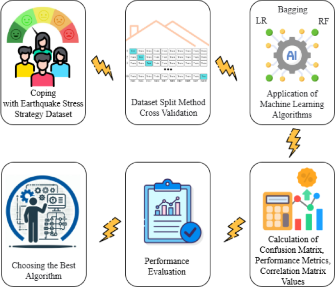 Fig. 2
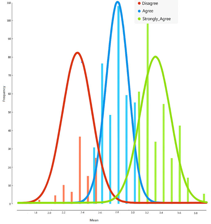
Threshold-based frequency distributions.
Table 2 Sample confusion matrix notation and Explanations.
Disagree (This person disagrees with the Coping with Earthquake Stress Strategy).
Agree (This person agrees with the Coping with Earthquake Stress Strategy).
Strongly agree (This person strongly agrees with the Coping with Earthquake Stress Strategy).
The Logistic Regression algorithm was chosen as a fundamental method due to its high interpretability and suitability for multi-class classification problems. Ensemble algorithms such as Random Forest and Bagging were preferred for their robustness in handling the complex and non-linear relationships often observed in psychological data, their resistance to overfitting, and their ability to achieve high accuracy. These ensemble methods enhance model generalizability by reducing variance.
Confusion matrix and performance metrics
Confusion Matrix and Performance Metrics are basic tools used to evaluate and compare the performance of artificial intelligence algorithms. These tools are used to determine how accurately the model works in classification processes and prediction processes20.
It is a table used to evaluate the performance of artificial intelligence algorithms. The table provides 4 pieces of information: TP, TN, FP and FN. According to this information, it can be observed which types of errors the algorithm makes and in which classes it is successful21,22,23. The sample confusion matrix representation and explanations in this study are presented in Table 2. The calculation of TP, TN, FP and FN values are presented in Table 3.
Table 3 The calculation of TP, TN, FP and FN values.
It consists of statistical metrics used in artificial intelligence methods and data science to measure how well the model performs24. These metrics are used to evaluate the accuracy, precision, errors or overall performance of the model25,26. In this study, accuracy, precision, recall and F1-score metrics are used. The descriptions and formulas of the metrics used are given in Table 4.
Table 4 Descriptions and formulas of performance metrics and Matthews correlation Coefficient.
Four main performance metrics are used to evaluate the success of the model. Accuracy represents the ratio of correct predictions made by the model to the total number of predictions. Precision indicates the proportion of correctly predicted positive results among all positive predictions. Recall shows how well the model identifies the actual positive cases. The F1-Score is the balanced average of precision and recall, used to measure the overall performance of the model. The formulas for these metrics are presented in Table 4.
Matthews correlation coefficient (MCC)
Matthews Correlation Coefficient (MCC) is a robust and comprehensive statistical measure used to evaluate the performance of classification models. It is especially valued for providing reliable results on imbalanced datasets. Unlike basic metrics such as accuracy, MCC takes into account true positives, true negatives, false positives, and false negatives simultaneously, offering a more nuanced assessment27. Its values range from − 1 to + 1, where + 1 indicates perfect classification, 0 corresponds to random guessing, and − 1 signifies complete misclassification. While commonly applied in binary classification problems, MCC also has generalized versions suitable for multi-class classification. By reflecting the overall balance of performance across all classes, MCC provides a fair and holistic evaluation of a model. In this study, the MCC values calculated for Logistic Regression, Random Forest, and Bagging algorithms were high, highlighting their accuracy and reliability as key indicators of model performance. The MCC values are shown in tables for algorithms.
Chi-square test (χ²)
Chi-Square Test (χ²): The Chi-Square test is a statistical method used in classification problems to determine whether a feature has a significant association with target classes. It is especially preferred when working with categorical data. This test helps identify the degree to which each feature is related to the classes, aiming to determine which features truly contribute to the classification process28.
The Chi-Square test can be applied directly to the data without the need for model training29. This allows for identifying significant variables independently of any specific model. As a result of the test, each feature receives a score that reflects its ability to discriminate between classes. Features with high scores are considered more important, while those with low scores can be deemed unnecessary and removed from the dataset.
This approach not only speeds up the model training process but can also improve accuracy. Additionally, its fast execution on large datasets is a significant advantage. The Chi-Square test is particularly effective and reliable as a preliminary analysis tool when working with categorical data or numerical data that can be discretized into categories.
As a result of the Chi-Square test, the three features contributing most significantly to the classification process were identified as CESS_10 (“I believe in fate and that it cannot be changed,” χ² = 130.674), CESS_13 (“I try to be more optimistic about life,” χ² = 85.521), and CESS_11 (“I fulfill my religious duties more often,” χ² = 79.574) (Table 5).
Table 5 Results of χ² variables.Correlation matrix
A correlation matrix is a symmetric square matrix that quantitatively represents the relationships between variables in a multivariate data set. This matrix contains the Pearson correlation coefficients between each pair of variables, ranging from − 1 to + 1, indicating the direction and strength of the relationship. The diagonal elements of the matrix are always 1 because the correlation of a variable with itself is strictly positive. The correlation matrix is used as a fundamental tool in multidimensional data analysis, factor analysis and various statistical modeling techniques, providing researchers with critical information in understanding the complex relationships between variables30,31.
−1: It represents a strong and negative correlation between two variables.
0: It represents the absence of a relationship between two variables.
1: It represents a strong and positive correlation between two variables
Cross validation
Cross validation is a statistical resampling method used to evaluate the performance of an artificial intelligence model on unseen data as objectively and accurately as possible. In this method, the data set is divided into k parts and one part at a time is used as a test set. The rest are used as the training set. This process is repeated for all parts and the performance of the model is measured at each iteration. The overall performance of the model is determined by averaging the results. This approach helps to understand how the model performs on different data subsets and helps to obtain more reliable results22,32,33. Cross validation is presented in Fig. 3. In this study, stratified folds were intentionally not used due to the relatively small size and clustered nature of the dataset, which could lead to overly homogeneous folds and affect model training. Instead, we used random folds to better reflect the natural variability of the data.
Fig. 3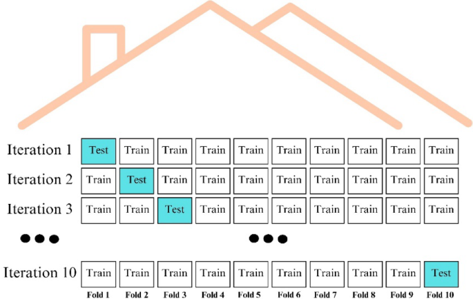 Artificial intelligence models
Artificial intelligence models are computer systems designed to perform various tasks. These models try to mimic human intelligence and demonstrate advanced capabilities in certain areas34. Logistic Regression, bagging and random forest algorithms were used in this study.
Logistic regression
Logistic regression is a statistical method and artificial intelligence algorithm used in classification problems. It is mainly used to model the relationship between independent variables and a categorical dependent variable. It uses the logistic function to transform the input variables into a probability value between 0 and 1. This probability usually represents the probability of an event occurring or belonging to a class. Logistic regression is widely used, especially in binary classification problems, but can also be adapted to multiclass problems35,36,37.
Bagging
It is an ensemble learning method and is used to improve prediction performance. In this model, random samples are taken from the original dataset and an independent model is trained on each sample. Then, the predictions of all models are combined to form a prediction. Voting is used for classification problems and averaging for regression problems38,39.
Random forest
Random Forest is a powerful artificial intelligence algorithm that is one of the ensemble learning methods and combines a large number of decision trees. This algorithm is based on the bagging method and additionally uses feature randomization. Each decision tree is trained on a randomly selected sample from the original dataset and a randomly selected subset of features is used at each node40. This approach increases the diversity of the model and reduces the risk of overlearning. In the prediction phase, the results of all trees are combined. Majority voting is used for classification and averaging is used for regression. Random Forest has the advantages of high accuracy, good generalization ability and applicability to different types of data26,41,42.