
We have calculated RPA spectra for all materials in the IPA database24 that have at most 8 atoms in the unit cell, i.e., a total of about 6000 spectra. The structures were originally taken from the Alexandria database of theoretically stable materials25. They include semiconducting and insulating compounds that contain only main group elements from the first five rows of the periodic table, have a distance from the convex hull less than 50 meV times the number of atoms in the unit cell, and a band gap greater than 500 meV. The data spans a wide range of crystalline systems, covering, e.g., common binary and ternary semiconductors and insulators, but also more exotic compounds such as layered two-dimensional systems and noble gas solids. A visualization of the elemental diversity of the data is given in Supplementary Fig. 3 and Supplementary Note 3. Additional computational details for the ab initio calculations are given in the “Methods” section. For the generated data, see the “Data availability” section.
For consistency, we employ the OPTIMATE architecture of GATs as in Ref. 18. The model is sketched in Supplementary Fig. 2 and takes as input a crystal structure and outputs a frequency-dependent optical property. An input crystal structure is first converted into a multigraph with the corresponding element encoded on each node and distances between atoms encoded on each edge. The model itself consists of a multilayer perceptron which acts on each node separately to process the elemental information, followed by three layers of message passing using the improved Graph Attention Operator of Ref. 23. Node-level information is then pooled using softmax vector attention to obtain a single high-dimensional vector which characterizes the material18. This vector is then passed through another multilayer perceptron to obtain the target optical property. The optical property itself is represented as a 2001-element vector, which corresponds to the optical property sampled in 10 meV steps from 0 eV to 20 eV. We refer to the original publication18 for a more detailed description of its architecture.
In this work, we focus on models trained to predict the imaginary part of the trace of the frequency-dependent dielectric tensor ε(ω). The imaginary part of the dielectric function determines together with the refractive index n the absorption spectra α(ω) via
$$\alpha (\omega )=\frac{\omega }{c}\frac{{{\rm{Im}}}(\varepsilon (\omega ))}{{{\rm{Re}}}(n(\omega ))}$$
(5)
where in general α, n and ε are all tensorial properties. The trace of these tensorial properties is an estimation of their polycrystalline average and allows for an easier handling of them26. We focus specifically on the dielectric function instead of, e.g., the refractive index or the absorption spectrum, as it is the direct result of the ab initio calculations discussed above, and is also usually reported in optical characterizations of materials, e.g., using ellipsometry.
We consider and compare two different strategies for learning the optical properties of materials at the RPA level, namely direct learning (DL) and transfer learning (TL). For DL, one initializes the weights of OPTIMATE randomly and trains directly on the expensive high-level optical spectra, i.e., the RPA spectra in our case. For TL, one trains OPTIMATE first on a large dataset of optical spectra of a lower theory level, i.e., in our case IPA, and then continues the training on a small number of optical spectra of a higher theory level, i.e., data calculated in the RPA. Since the RPA spectra in this work are calculated with a 300 meV broadening, we use the corresponding IPA-OPTIMATE model, i.e., the one trained on the trace of the imaginary part of the dielectric function under IPA, \({{\rm{Im}}}({\overline{\varepsilon }}_{{{\rm{IPA}}}})\), with a 300 meV broadening. In this process, we retrain all learnable parameters of the base model18 starting from the IPA weights, because, in contrast to many other applications involving, e.g., large language models, the additional cost is negligible, and recent publications21,27 have shown that this is generally the best strategy for transfer learning graph neural networks for materials science, even when transfer learning between closely related properties. To avoid data leakage, we reuse the training, validation, and test sets used in the original training of OPTIMATE18, leaving us with a total training set of 4610 materials and associated spectra, a validation set of 603 materials and a test set of 639 materials. This ensures that the transfer-learned OPTIMATE model has not seen any of the materials in the RPA validation and test set during its original training on IPA data. To compare the data efficiency of the DL and TL, we divided the training set into randomly formed subsets of 100, 300, 1000, 3000, and 4610, i.e., the entire training set. To ensure a fair comparison, we optimize both the architecture and the hyperparameters of the OPTIMATE models used for the DL strategy. The architecture of the OPTIMATE models used for the TL strategy is necessarily kept fixed, so only the hyperparameters of the optimizer are tuned. The training procedure, the selection of the final models, and their hyperparameters are described in more detail in the “Methods” section.
As error metric to compare two spectral properties X(ω) and Y(ω) in a scale-invariant way, we define the similarity coefficient (SC)28
$${{\rm{SC}}}[X(\omega );Y(\omega )]=1-\frac{\int\left\vert \right.X(\omega )-Y(\omega )\left\vert \right.\,d\omega }{\int\left\vert \right.Y(\omega )\left\vert \right.\,d\omega }$$
(6)
In addition, we use the mean square error (MSE)
$${{\rm{MSE}}}[X(\omega );Y(\omega )]=\frac{1}{{\omega }_{{\max }}}\int|X(\omega )-Y(\omega ){|}^{2}\,d\omega$$
(7)
as another measure of similarity between spectra. During training, we use the L1 loss, outside of machine learning commonly referred to as the mean absolute error (MAE):
$${{\rm{MAE}}}[X(\omega );Y(\omega )]=\frac{1}{{\omega }_{{\max }}}\int\left\vert \right.X(\omega )-Y(\omega )\left\vert \right.\,d\omega$$
(8)
We use a shorthand, e.g., SC[RPADFT; IPADFT] to refer to \({{\rm{SC}}}[\overline{\varepsilon }{(\omega )}_{{{\rm{DFT}}}}^{{{\rm{RPA}}}};\overline{\varepsilon }{(\omega )}_{{{\rm{DFT}}}}^{{{\rm{IPA}}}}]\), i.e., in this example, the SC between \(\overline{\varepsilon }\) obtained via DFT using the RPA in reference to \(\overline{\varepsilon }\) obtained via DFT using the IPA.
Comparison of direct learning and transfer learning
The main results of this work are summarized in Figs. 2 and 3, which compare both learning strategies for various training-set sizes. The examples in Fig. 2 show that DL on a small dataset of 300 materials leads to noisy, unphysical spectra consisting mostly of a single broad peak (which, perhaps surprisingly, is often more or less correctly positioned). In contrast, the TL strategy results even for small trainings sets already in realistic spectra, showing quite good quantitative agreement. For larger training set sizes, e.g., for 4610 training materials as shown, both strategies lead to a similar prediction accuracy. This is shown in more detail in Fig. 3, where the median SC, Eq. (6), and the median MSE, Eq. (7), of the test set for various training set sizes are compared between both strategies. Both error measures are similar for both strategies when the training set is large enough, but the transfer learning strategy already achieves similar error measurements with just 300 materials as the direct learning strategy with about 3000 materials. All models perform better than the possible baseline of just using the IPA spectra. Numerical values for the IPA baseline, i.e., \({G}_{\max }=0\), as well as for the non-converged \({G}_{\max }=2000\) mRy are given in Supplementary Table 4. Parity plots for both strategies trained on 300 and 4610 materials are shown in Supplementary Fig. 4 and Supplementary Note 4 and yield similar results.
Fig. 2: Spectra as predicted via DL and TL after training on datasets of different sizes.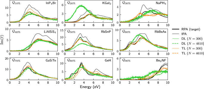
Spectra of nine materials selected at the 10% quantile, the 20% quantile, …, the 80% quantile and the 90% quantile of the test set ordered according to the similarity coefficient SC[IPADFT; RPADFT]. All calculated or predicted spectra were obtained for a larger energy range of 0–20 eV, but are shown for a smaller energy range to emphasize the differences. All IPA spectra (thin black) differ considerably from the RPA spectra (thick black line). The latter are reasonably well predicted via transfer learning (orange) on large (thick dashed lines, 4610 materials) or even small (thin lines, 300 materials) trainings sets, whereas direct learning (green) on 300 materials yields unphysical, overly broad and very noisy spectra. Much larger training sets would be required for good and physically sensible results with direct learning. N in the legend indicates how many materials were used for training.
Fig. 3: Comparison between DL and TL for different training set sizes.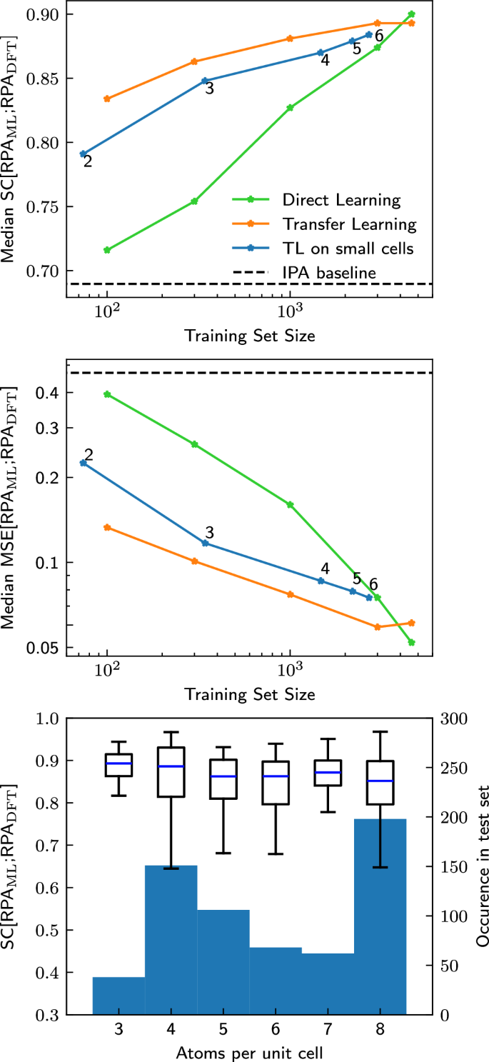
Median SC (top) and median MSE (middle) on the test set for direct learning (green) and transfer learning on subsets of different size of the training set (orange) or exclusively on systems with small unit cells (blue) as a function of the training-set size (indicated by the stars). Using the DFT-calculated IPA spectra as a proxy for the RPA spectra (taken over the entire test set) is given as a baseline in the black dashed line. The small number next to each data point on the blue curve indicates the maximum number of atoms per primitive unit cell. Bottom: Boxplot of the distribution of SC[RPAML; RPADFT] on the full test set after transfer learning only on materials with up to 4 atoms per primitive unit cell. The test set is split up by number of atoms per primitive unit cell. The blue center line of the boxplot shows the median, the boxes show the interquartile range, and the whiskers extend out from the box to the furthest point lying within 1.5 times the interquartile range. As can be seen, transfer learning only on materials with few atoms per unit cell generalizes to materials with more atoms per unit cell. The number of materials in the test set with a given number of atoms per primitive cell is given by the background histogram. No materials with 1 and only very few materials with 2 atoms per primitive unit cell are present in the test set.
In short, transfer learning allows accurate quantitative prediction of spectra with a training set of only the order of 100–1000 materials. Furthermore, we believe that the observed convergence in model performance between both strategies is likely due to the RPA training set approaching the size of the initial IPA training set for the model, as it is often observed in TL that as the underlying training set increases, TL accuracies also improve21.
Hitherto, we have seen that a few (about 300) numerically more expensive RPA calculations are sufficient to retrain the OPTIMATE IPA model. Now, we turn to the question of whether we can pick particularly cheap examples for the TL strategy. So far, the data used for transfer learning consisted of random subsets of the data used to train the underlying model. As discussed in the introduction, almost all computational techniques scale unfavorably with the system size (often \({{\mathcal{O}}}({N}^{3})\) or worse), as opposed to graph neural networks, which generally scale as \({{\mathcal{O}}}(N)\), with N being the number of atoms in the unit cell. If instead of using a random subset of the original training data one could instead only use data from small unit cells, one might significantly reduce computational time. We therefore transfer learn the IPA model on a subset of the training data consisting of only the materials with at most 2, 3, 4, 5 and 6 atoms per primitive unit cell (using the optimal hyperparameters for a training set size of 1000). The results are shown as blue lines in Fig. 3 and they are impressive: Even with TL on materials which only contain up to 2 atoms per primitive unit cell, which are only around 60 materials in total, a median SC of 0.8 is achieved. With only up to 4 atoms per primitive unit cell, i.e., around 1500 materials, median MSEs below 0.1 and SC above 0.85 are achieved.
One could speculate that learning on small cells primarily improves the performance on other small cells, while not improving the errors on larger cells. But that is not the case: Fig. 3 (bottom) shows the SC for the materials in the test set grouped according the number of atoms per primitive unit cell, evaluated for the model trained on cells with up to 4 atoms per primitive unit cell. The error for all unit cell sizes is equally small, i.e., even when transfer learning only on materials with small cells, the properties of materials with larger cells can be predicted equally as well. If this were a general result, it would be very encouraging for related future work, e.g., climbing further rungs towards accurate prediction of experimental spectra.
Deeper investigation into transfer learning
We further investigate the success of transfer learning. Figure 4 quantifies the observations that are suggested by the illustrative examples of Figs. 2 and 3. We start with the one-dimensional histograms marking rows and columns. The most important observation is that the TL-RPA predicts the ab initio DFT-RPA (see panel b) about as well as the underlying ML-IPA model18 predicts the DFT-IPA (panel d). Even the poorly trained DL prediction (a) is not worse than the possible baseline of simply using the DFT-calculated IPA spectrum (c), see also Fig. 3.
Fig. 4: Correlations between various similarity coefficients on the test set after training on 300 materials.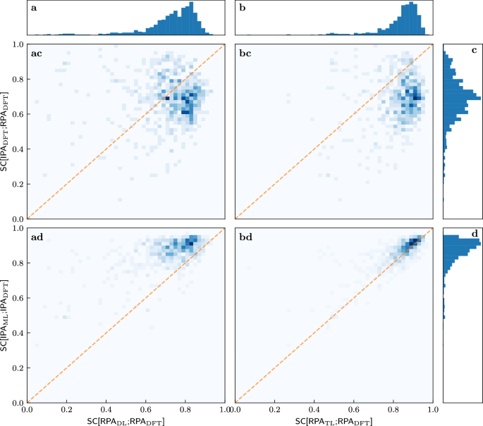
The columns refer to SC[RPADL;RPADFT] a and SC[RPATL;RPADFT] b, while the rows refer to SC[IPADFT;RPADFT] c, SC[IPAML;IPADFT] d. The histogram in the first row shows that the ab initio IPA spectra are only a rough approximation of the ab initio RPA spectra. The histogram in the second row reproduces the observation of Ref. 18 that very good ML predictions of the DFT-IPA spectra are possible. The histograms in the top panels show that TL predicts the ab initio RPA spectra much better than DL. The two-dimensional histograms in the center show the correlations between the SCs defining columns and rows. All SCs are evaluated on the test set. The dashed orange line marks the angle bisector.
The first row of the two-dimensional histograms in Fig. 4 addresses the question of whether the quality of ML prediction on the RPA level depends on how much the ab initio RPA and IPA spectra actually differ, in other words, whether the ML predictions are worse for difficult cases with small SC[IPADFT;RPADFT]. Obviously, there is no (strong) correlation, the models predict RPA spectra more or less well, regardless of how much the RPA changes the IPA spectra. While this may be obvious for the direct learning strategy (panel ac), this is far from obvious for the transfer learning strategy (panel bc), which starts training from a model which predicts the IPA spectra.
Examining the bottom row of two-dimensional histograms in Fig. 4 reveals an even more interesting fact: There is a correlation between whether the models can predict the RPA spectra and whether another model can predict the IPA spectra. Most peculiarly, the numerical values of the corresponding SCs are almost the same when transfer learning already on small datasets (panel bd). This means that the RPA spectra for a given material can be predicted just as well as the IPA spectra. This correlation is made even more clearer when training on 4610 materials, and the same agreement is recovered for DL on such dataset sizes, see Supplementary Fig. 1. One might have expected—wrongly, as it turns out—that the RPA spectra would be more difficult to predict than the IPA spectra, since they include additional physical effects.
From a machine-learning point-of-view, the fact that RPA and IPA spectra are equally well predictable might not be surprising, by—perhaps overly reductionistly—assuming the models treat the RPA spectra compared to the IPA spectra as just another curve defined in a learned materials space. As we have shown recently, the models construct expressive internal representations of the material space29. Therefore, we propose that the models reconstruct very general features of the material space (similarity between materials in general) contained in the training set before converting them to a specific property (in this case the RPA dielectric function).
To investigate this further, we compare in Fig. 5 how well each material is predicted by both strategies for various training set sizes. Again, TL performs much better than the DL strategy for the small training set. Both strategies perform similarly well for the large training set, where an almost linear correlation exists, with possibly a slight advantage for DL. Thus, not only is the predictability between the IPA spectra and the RPA spectra strongly correlated, but the predictability of the RPA spectra for a given material is also approximately independent of the training strategy employed (once the training set is large enough).
Fig. 5: Comparison between TL and DL for different training set sizes.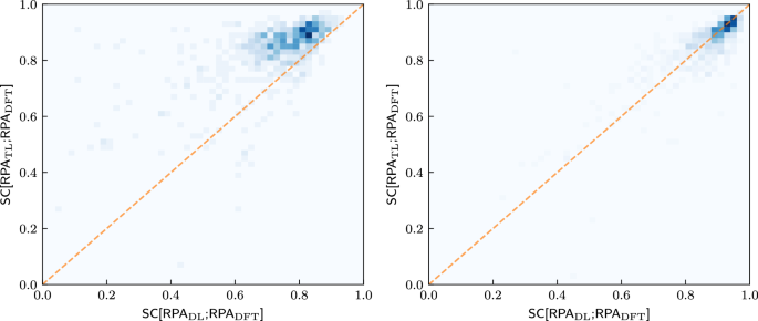
2D-Histograms comparing the similarity coefficients SC[RPAS; RPADFT], S = DL, TL, on the test set for both training strategies after training on 300 (left) and 4610 (right) materials. The orange line marks the angle bisector.
Learning the similarity
Finally, we investigate whether it is possible to directly predict the similarity between the DFT-IPA spectra and the DFT-RPA spectra. This could be useful, e.g., when deciding which level of theory is necessary to model a given material. For this purpose, we train a model with the same architecture as OPTIMATE18, except that we change the output dimension of the final output layer from a dimension of 2001 to 1, i.e., the dimension of the SC (see Supplementary Note 5 for training details). The results are shown in Fig. 6. As can be seen, the similarity coefficient between the IPA and the RPA spectra can be predicted extremely well, with a mean and median absolute error of 0.026 and 0.018, respectively. This bodes well for further studies. One might, e.g., design a high-throughput workflow which incorporates such models to effectively select the highest level of theory necessary to describe the properties for a given material, saving valuable computational resources.
Fig. 6: Predicting the similarity between the RPA and the IPA.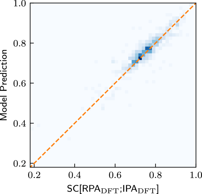
Prediction of SC[RPADFT; IPADFT] on the test set after training on the entire training set. The straight line marks the angle bisector.
Which materials are well described by the IPA already?
The database presented in this work is the largest database of well-converged RPA calculations that we are aware of. Apart from being of direct practical use, one might hope to glean physical insight from such a database, for example by asking “Which (classes of) materials are well described by the IPA already”, or framed in another way, “Which materials possess very strong local-field effects”. From a theoretical point of view, the IPA is in essence a maximal truncation of a basis set (see Eq. (2)), and treats the susceptibility as being constant over the entire unit cell3,22. How correct this is obviously varies from material to material, and one might attempt to correlate it with the anisotropy of the electron density, for example. We instead make use of our descriptor SC[RPADFT;IPADFT] for an initial attempt to answer this question. Manually inspecting the materials with the lowest similarity SC[RPADFT;IPADFT] (see “Code availability” statement) reveals that most of these materials are ones that either consist of condensed weakly bound clusters or molecules (e.g., S8-rings, N2O, CO2, N2) or materials including many halogen or nitrogen atoms. The response of the former class is spatially inhomogeneous more or less by definition. Intuitively, strong local-field effects of the latter class might be explained by its very electronegative elements, which lead to unequal charge distributions and anisotropic screening. However, an explanation of low SC[RPADFT;IPADFT] values based on electronegativity alone suggests small SC values for oxides as well, which is not clearly supported by the data. Direct inspection of the materials with the largest SC[RPADFT;IPADFT] did not show any obvious material clusters.
We therefore proceed with an alternative approach. We extract the latent activations for the SC[RPADFT;IPADFT]-prediction network after the pooling step and reduce them to two dimensions using the UMAP algorithm30 (for details, see “Methods” section). As we have previously shown, a UMAP after the pooling step (on our specific architecture) generally clusters according to chemical principles and can be interpreted as a map of the chemical space from the point of view of the trained model29. The resulting UMAP is shown in Fig. 7, and one can clearly see that the materials with extremely low similarity cluster (materials with many halogen atoms to the right, azides, nitrates etc. to the lower left), while materials with average or high similarity are more spread out. The identity of each dot (i.e., each material) is identified via an interactive version of this UMAP with which one can investigate where each material is placed (see “Data availability” section).
Fig. 7: UMAP of latent embeddings of SC-prediction model, colored by true SC.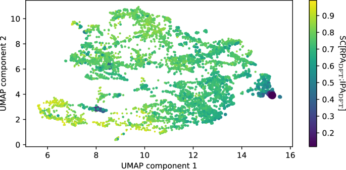
Each dot represents a material. The color and size of each dot are related to the SC, with larger/darker dots showing less similarity between RPA and IPA. There are two distinct clusters of very low similarity. The right purple cluster consists of compounds with extreme amounts of halogens (e.g., KF3, RbBrF6, XeF2, etc.), while the purple cluster closer to the lower left corner consists mostly of azides, nitrates and other nitrogen-containing compounds (e.g., NaN3, LiNO3, N2, etc.).