
We begin by abstracting an isotropic real solid as a homogeneous continuum model embedded with some scatterers. The system’s vibrations can be treated as the elastic phonons resonating with local modes. There are two system-averaged length scales: the typical size ξ of scatterers and the characteristic mean free path \(\ell\) (or mobility distance) of the scattering, jointly modulating the degree of resonance. In terms of the displacement field u, the full dynamics of the system can be described by
$${\bf{M}}\ddot{{\bf{u}}}+{\bf{H}}\dot{{\bf{u}}}+{\bf{K}}{\bf{u}}=0$$
(1)
where M, H and K are the mass matrix, viscous damping matrix and stiffness matrix, respectively. Owing to the complexity, equation (1) is impossible to solve analytically. Usually in underdamped states, H is often assumed to be a linear combination of M and K. If ignoring phonon–phonon interactions, these matrices become positive-definite and diagonal. Thus, equation (1) can be decomposed into a set of damped harmonic phonons:
$${m}_{\lambda }{\ddot{u}}_{\lambda }+{\eta }_{\lambda }{\dot{u}}_{\lambda }+{k}_{\lambda }{u}_{\lambda }=0$$
(2)
where \({m}_{\lambda }\), \({\eta }_{\lambda }\) and \({k}_{\lambda }\) are the mass, viscosity and stiffness, respectively; the subscript λ = 1…3N denotes the numbering of phonons. Then, we assume that equation (2) has a solution of the form \({u}_{\lambda }(t)={G}_{\lambda }(\omega ){{\rm{e}}}^{-{\rm{i}}\omega t}\), where \({G}_{\lambda }(\omega )\) is the ω-dependent Green’s (response) function
$${G}_{\lambda }(\omega )=\frac{1}{{\varOmega }_{\lambda }^{2}-{\omega }^{2}+{\rm{i}}\omega {\varGamma }_{\lambda }}$$
(3)
where \({\varOmega }_{\lambda }=\sqrt{{k}_{\lambda }/{m}_{\lambda }}\) and \({\varGamma }_{\lambda }={\eta }_{\lambda }/{m}_{\lambda }\). This single-degree-of-freedom Green’s function can be formally generalized to a three-dimensional \(q\)-dependent version31,32,33,34 as
$$G(q,\omega )=\frac{1}{{\varOmega }^{2}(q)-{\omega }^{2}+{\rm{i}}\omega \varGamma (q)}$$
(4)
where \(\varOmega (q)\) and \(\varGamma (q)\) are related to the real and imaginary parts, respectively, of the self-energy function that takes the phonon–phonon interactions into account19,28. Considerable efforts have been spent in the past decades to obtain the exact expression for the self-energy function by resorting to various methods such as the self-consistent Born approximation19,20 and the Taylor expansion29,30,35.
Here we revisit \(\varGamma (q)\) from the perspective of phonon scattering. When an extended phonon (elastic wave) interacts with scatterers, its propagation becomes damped. This scattering process involves the absorption and re-radiation of phonons, mathematically corresponding to the second-order derivative of \({u}_{\lambda }(t)\) with respect to t. We, thus, obtain the response of the λth scattering wave, \({\ddot{u}}_{\lambda }(t)=-{\omega }^{2}{G}_{\lambda }(\omega ){{\rm{e}}}^{-{\rm{i}}\omega t}\), with its amplitude
$${A}_{{\rm{s}}}={\omega }^{2}|{G}_{\lambda }(\omega )|=\frac{{\omega }^{2}}{\sqrt{{({\varOmega }_{\lambda }^{2}-{\omega }^{2})}^{2}+{\varGamma }_{\lambda }^{2}{\omega }^{2}}}$$
(5)
According to the acoustics principles36, the scattering intensity \({W}_{\lambda }\) is proportional to the scattering cross-section and the square of amplitude, that is,
$${W}_{\lambda }\propto {\rm{\pi }}{\xi }^{2}{A}_{s}^{2}={\rm{\pi }}{\xi }^{2}\frac{{\omega }^{4}}{{({\varOmega }_{\lambda }^{2}-{\omega }^{2})}^{2}+{\varGamma }_{\lambda }^{2}{\omega }^{2}}$$
(6)
Interestingly, equation (6) resembles that for the scattering of electromagnetic waves by bound electrons37 or sound waves by bubbles38. By summing \({W}_{\lambda }\) over all phonons (Extended Data Fig. 1), we can obtain the total scattering intensity of the system as
$${W}_{{\rm{t}}}=\mathop{\sum }\limits_{\lambda =1}^{3N}{W}_{\lambda }\approx \alpha {\rm{\pi }}{\xi }^{2}\frac{{\omega }^{4}}{{({\varOmega }_{0}^{2}-{\omega }^{2})}^{2}+{\bar{\varGamma }}^{2}{\omega }^{2}}$$
(7)
where α is a coefficient and \({\varOmega }_{0}\) and \(\bar{\varGamma }\) are the system-averaged eigenfrequency and damping, respectively. For scatterers, \(\omega\) donates the frequency before scattering, so the scattering-free phonons can be regarded as ‘external’ linear excitations (\(\omega =cq\), where c is the wave velocity). Therefore, equation (7) transforms into
$${W}_{{\rm{t}}}=\alpha {\rm{\pi }}{\xi }^{2}\frac{{q}^{4}}{{({q}_{0}^{2}-{q}^{2})}^{2}+{q}^{2}{\theta }^{2}}$$
(8)
where \({q}_{0}={\varOmega }_{0}/c\) and \(\theta =\bar{\varGamma }/c\). In reciprocal space, \({q}_{0}\) is related to the typical scatterer size by \({q}_{0}=2\pi /\xi\), and \(\theta\) is related to the characteristic mean free path of scattering by \(\theta =2\pi /\ell\). Obviously, a smaller q0 corresponds to a larger ξ, whereas a smaller \(\theta\) indicates a longer \(\ell\). Given that phonon damping directly results from scattering, \(\varGamma (q)\) of the system can be approximately proportional to the scattering intensity Wt:
$$\varGamma (q)\propto {W}_{{\rm{t}}}={\varGamma }_{0}\frac{{q}^{4}}{{({q}_{0}^{2}-{q}^{2})}^{2}+{q}^{2}{\theta }^{2}}$$
(9)
where \({\varGamma }_{0}=\alpha \pi {\xi }^{2}\). In the following, q0, q and \(\theta\) are each normalized by the Debye wavenumber \({q}_{\rm{D}}=2\pi /a\), with \(a\) being the average atomic spacing. We, thus, obtain the dimensionless \({q}_{0}=a/\xi\) and \(\theta =a/\ell\). Usually, both ξ and \(\ell\) are about 1–5 average atomic spacing14,39,40; thus, the range of \({q}_{0}\) and \(\theta\) is preliminarily set as 0.2 to 1.
At the long-wavelength limit (\(q\to 0\)), \(\varGamma (q)\) described by equation (9) follows the famous Rayleigh damping law; increasing q to \({q}_{0}\), equation (9) becomes \(\varGamma (q)\sim {q}^{2}\), that is, Mie damping law. This theoretical prediction is consistent with experiments22,23,41 and numerical calculations19. To the best of our knowledge, this is the first time that such a transition of phonon damping has been theoretically predicted. It is noted that the present \(\varGamma (q)\sim {q}^{2}\) law in the high-\(q\) region is different from diffusive \({q}^{2}\) damping, as recently revealed35, and the latter results from non-affine motions and occurs far below the Rayleigh region. We also compare our model with \(\varGamma (q)\sim -{q}^{4}\,\mathrm{ln}\,q\) reported in ref. 21 by fitting the damping data of atomistic-simulated binary soft-sphere glasses42. Figure 1a shows that in the low-q region, both longitudinal and transverse \(\varGamma (q)\) data can be well fitted by equation (9) (red solid lines) and \(-{q}^{4}\,\mathrm{ln}\,q\) (blue solid lines). However, in the high-q region, the \(-{q}^{4}\,\mathrm{ln}\,q\) scaling breaks down, but our model still works. It must be pointed out that the deviation of the transverse data from the theoretical prediction is due to the sample’s finite-size effects21. This deviation disappears for a three-dimensional inverse power-law glass of up to 4,000,000 particles43 (Extended Data Fig. 2). Again, our model shows better prediction than \(-{q}^{4}\,\mathrm{ln}\,q\) scaling, which is further tested by fitting the \(\varGamma (q)\) data of NiZr crystalline alloy44 and densified SiO2 glass45 (Supplementary Fig. 1). These results prove the robustness and universality of equation (9).
Fig. 1: Theoretical model of VDOS.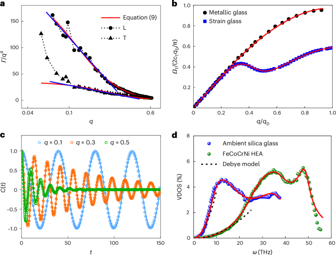
a, Comparison between the damping data of atomistic-simulated binary soft-sphere glasses21 with equation (9) (red solid lines) and the –q4lnq law (blue solid lines). b, Comparison between the calculated TA dispersion (equation (11)) with the experiments of Zr46Cu46Al8 metallic glass measured by using inelastic neutron scattering48 and the simulations of Zr95.5Ni4.5 strain glass15; the fitting parameters are listed in Supplementary Table 1. c, Velocity autocorrelation function C(t) (equation (12)) at q = 0.1, q = 0.3 and q = 0.5, which is well fitted by \(\exp (-\varGamma (q)t/2)\cos(\varOmega (q)t)\). d, Comparison between the theoretical VDOS (equation (13)) with the experimental data of an ambient silica glass7 and FeCoCrNi HEA49, and the fitting parameters are listed in Supplementary Table 2. The dashed lines indicate the Debye model.
We next discuss the eigenfrequency \(\varOmega (q)\) under damping \(\varGamma (q)\). For a damped-elastic solid, the phonon kinetic energy is proportional to the square of eigenfrequency, that is, \({E}_{k}(q)\propto {\varOmega }^{2}(q)\). According to the displacement of a damped plane wave46, we can write \({E}_{k}(q)\approx {E}_{0}(q)\exp (-\varGamma (q)/c{q}_{D})\), where \({E}_{0}(q)\propto {\varOmega }_{\rm{lattice}}^{2}(q)\) is the phonon kinetic energy of a damping-free crystal. Generally, \({\varOmega }_{\rm{lattice}}(q)\) has a sinusoidal form47
$${\varOmega }_{\rm{lattice}}(q)=\frac{2c{q}_{\rm{D}}}{\pi }\,\sin \left(\frac{\pi q}{2{q}_{\rm{D}}}\right)$$
(10)
This formula is derived from the standard result of one-dimensional chains, but still works as an approximation for three-dimensional lattices9. Inserting equation (10) into \({E}_{k}(q)\), we can derive the expression of \(\varOmega (q)\) as
$$\frac{\varOmega (q)}{2c{q}_{\rm{D}}/\pi }=\,\sin \left(\frac{\pi q}{2{q}_{\rm{D}}}\right)\exp \left(-\frac{\varGamma (q)}{2c{q}_{\rm{D}}}\right)$$
(11)
where the sinusoidal term on the right-hand side describes the inherent softening near \({q}_{\rm{D}}\), which is further damped by the exponential term (\(\varGamma (q)\) is given by equation (9)). Equation (11) highlights the theoretical relationship between the softening and damping of phonons, which is supported by existing experimental and numerical evidences21,22,23. Figure 1b presents the perfect agreement between the predicted TA dispersion (red solid lines) and the experimental data of Zr46Cu46Al8 metallic glass measured by using inelastic neutron scattering48, and the simulated data of Zr95.5Ni4.5 strain glasses15. Both the sinusoidal-type inherent global softening and the local softening can be captured by our theoretical model. Previously, only the Taylor expansion to higher orders could achieve this prediction30.
On the basis of equation (11), we can further evaluate the phonon propagation and damping by calculating the velocity autocorrelation function as
$$C(t)={k}_{\rm{B}}T\mathop{\sum }\limits_{q}\int \delta (\omega -\varOmega (q))\cos (\omega t){\rm{d}}\omega$$
(12)
where \({k}_{\rm{B}}\) is the Boltzmann constant and \(T\) is the temperature (here \(T\) = 300 K, and the choice of \(T\) does not influence the analysis as \({k}_{B}T\) normalization is carried out on \(C(t)\)). Figure 1c shows the normalized \(C(t)\) of the transverse excitation with q = 0.1, q = 0.3 and q = 0.5 when \({q}_{0}=0.5\) and θ = 0.8. Clearly, the long-wavelength phonon (q = 0.1) retains its rigid propagation characteristic. Increasing q to 0.5 (the wavelength is the same size as the scatterer), a noticeable oscillatory decay can be observed. In essence, the shorter the wavelength (relative to the scatterer size) of the phonon, the more severe the damping and scattering. Besides, all \(C(t)\) values can be well fitted by \(\exp (-\varGamma (q)t/2)\cos(\varOmega (q)t)\) (solid lines), which is proposed in ref. 21 and formally consistent with equation (11). It further supports that equation (12) effectively describes the propagation and damping of phonons with different wavelengths.
The known \(\varGamma (q)\) and \(\varOmega (q)\) allow for a quantitative calculation of the VDOS. The VDOS can be extracted from the imaginary part of the Green’s function (equation (4)) as
$$g(\omega )=-\frac{2\omega }{\pi {q}_{\rm{D}}^{3}}{\int }_{\!0}^{{q}_{\rm{D}}}\text{Im}[2{G}_{{\rm{T}}}(q,\omega )+{G}_{{\rm{L}}}(q,\omega )]{q}^{2}{\rm{d}}q$$
(13)
where the subscripts T and L represent the transverse and longitudinal branches, respectively. As shown in Fig. 1d, the experimental VDOS data of almost the entire frequency spectrum (red solid lines), including ambient silica glass7 and FeCoCrNi HEA49, can be well described by equation (13). It is noted that the two (transverse and longitudinal) peaks in the VDOS of HEA are also captured by our model. For comparison, the dashed lines indicate the Debye model that only satisfies the low-\(\omega\) limit. With increasing \(\omega\), the Debye model shows an obvious deviation from experimental data, but our model does not.