Global loss of mountain vegetated landscapes and its impact on biodiversity conservation

Mapping global mountain vegetated landscapes

We first mapped MVL in 2000 as a base map from which to estimate changes. To do so, we combined a global land-cover dataset in 2000 with a global mountain dataset. For land cover, some moderate spatial resolution products exist, such as the MODIS Land Cover Type from 2001 to 2016 (500 m), the ESA Climate Change Initiative (ESA-CCI) from 1992 to 2015 (300 m), Copernicus Global Land Cover Layers (CGLS-LC100) from 2015 to 2019 (100 m), Finer Resolution Observation and Monitoring of Global Land Cover product (FROM-GLC) in 2010, 2015 and 2017 (30 m/10 m), Globeland30 in 2000, 2010 and 2020 (30 m), global 30 m land cover classification with a fine classification system (GLC_FCS30D) in 2000 and 2020 (30 m) and ESA’s WorldCover in 2020 and 2021 (10 m)78,79,80,81. However, we chose GLC_FCS30D in our study mainly due to its high spatial resolution, suitable temporal resolution, fine classification system and more stable accuracy on a global scale compared to other 30-m global land-cover products82. The GLC_FCS30D product was produced by combining time series of Landsat imageries and high-quality training data from the Global Spatial Temporal Spectra Library on the Google Earth Engine cloud computing platform and presented at an approximately 30-m resolution80. The accuracy of GLC_FCS30D has been validated using numerous validation samples, with an overall accuracy of more than 81 %83,84 (available from Zenodo: https://doi.org/10.5281/zenodo.8239305), and it has been extensively used for a variety of applications45,85. For mountain delineation, commonly used global datasets include the United Nations Environment Programme-World Conservation Monitoring Centre (UNEP-WCMC) mountain inventory86 and the Global Mountain Biodiversity Assessment (GMBA)87,88 inventories (both standard and broad versions). After checking these mountain datasets, we found that the UNEP-WCMC dataset omits important mountain areas (e.g., southeastern Russia, central New Zealand, northern Norway) and overestimates some mountainous areas (e.g., northwestern China) (Supplementary Table 5). Likewise, the broad GMBA version incorporates not only mountainous terrain but also extends into adjacent landscapes88(Supplementary Table 5). On the other hand, the standard GMBA version (v2.0 standard) (https://www.earthenv.org/mountains) was better suited and addressed the aforementioned issues, which we thus chose in our study. This dataset delineates mountains covering ~ 18.2% of the Earth’s land surface (Supplementary Fig. 1).

To combine these datasets, we first converted the mountain boundary polygons into a grid image of 30 m resolution using the polygon to raster tool of ArcGIS. We then reclassified the GLC_FCS30D product into six land cover types following Zhang et al.80: cropland, impervious surface, forest, grassland, shrubland and other land. In this dataset, cropland is defined as land used for crop cultivation, including rain-fed croplands, herbaceous cover, and tree/shrub-covered croplands (e.g., orchards, plantations)80; impervious surface refers to hardened surfaces composed of artificial materials, including constructed materials (e.g., cement, asphalt and bricks) and artificially compacted surfaces (e.g., paved grounds, rocks and building foundations)80; forest, shrubland, and grassland are defined as land cover types dominated by trees, shrubs, and herbaceous plants, respectively. Forests include various types (e.g., evergreen broadleaved forest, deciduous broadleaved forest, and mixed-leaf forest); shrublands include both evergreen and deciduous types80. Following ecological principles, vegetation structure, the Intergovernmental Panel on Climate Change guidelines, and the Food and Agriculture Organisation Global Ecological Zones, these three classes represent the primary vegetated land cover types in global mountain ecosystems89,90,91. Therefore, we selected forest, shrubland, and grassland to define different vegetated landscapes, with all other classes designated as non-vegetated landscapes. We calculated mountain vegetated landscapes (MVL) by calculating spatial overlays between these vegetated landscapes with standardised mountain boundaries (GMBA v2.0), and defining all overlapping pixels as MVL. All calculations involving the map area were performed in WGS 84/Equal Earth Greenwich projection. Overall, we found a total area of approximation 18,681,548.8 km2 of MVL in 2000 (Supplementary Table 6).

Tracking global MVL loss(1) Human expansions-driven MVL loss

To track MVL loss since 2000 due to the expansion of human activities, we collected multi-source thematic datasets that quantify possible human activities in mountain areas. These included the impervious surface dataset (30 m resolution) and cropland dataset (30 m resolution) from 2000 and 2020, both of which are subsets of the GLC_FCS30D, as well as global mining distribution data (polygons). For global mining distribution data, we combined two recent global mining datasets from Maus et al.22 (total 44,929 polygons, covering 101,583 km²) and Tang et al.23 (total 74,548 polygons, covering 66,000 km2). These two datasets provide spatially explicit estimates of the area directly used for surface mining on a global scale (including large-scale and artisanal and small-scale mining), and the polygons cover all ground features related to mining activities (e.g., open cuts, tailing dams, waste rock dumps, water ponds, processing infrastructure). They were produced using remote sensing analysis of high-resolution, publicly available satellite imagery in recent years (e.g., around 2020; images with ≤ 10 m resolution in Google Earth and Sentinel-2) (details in refs. 22,23). The overall accuracies of these two global mining datasets calculated from the validation points were 88.3% (for Maus et al.22) (version 2, https://doi.org/10.1594/PANGAEA.942325) and ~ 92% (for Tang et al.23) (version 2, https://zenodo.org/records/7894216).

We merged the two global mining datasets to compensate for the potential omission of global mining areas from the different datasets using union analysis in ArcGIS 10.8. After merging, a combined global mining dataset was obtained (i.e., 81,962 polygons, covering 120,413 km2) (Supplementary Fig. 9). We then converted all polygons into a grid image of 30 m resolution using the polygon to raster tool of ArcGIS. To avoid overestimation of MVL loss caused by pixel overlap between datasets, we used spatial overlay analysis to detect overlapping pixels of impervious surface, cropland and mining areas. If there are overlapping pixels, we assigned their attributes to mining areas, because the mining data holds better spatial resolution and accuracy.

We quantified global MVL loss driven by human expansion according to the following rules:

(i) Human settlement growth

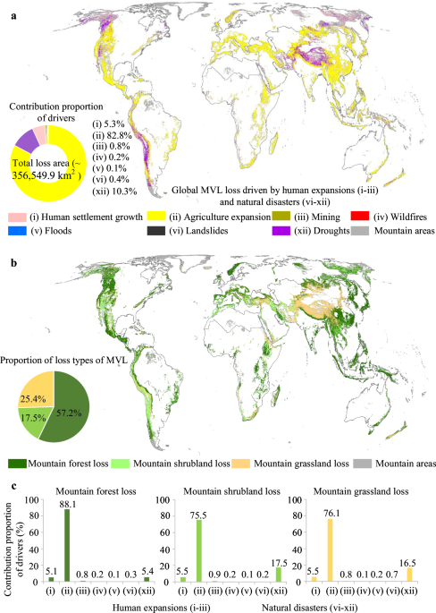
We used the expansion of impervious surface to reflect the growth of human settlements92,93. To do so, we used a pixel-level change detection method to identify the pixels that were impervious surface in 2020, but not in 2000. The MVL loss driven by human settlements denotes the pixels of MVL in 2000 that were transformed into human settlements by 2020 (Fig. 1a).

(ii) Agriculture expansion

We used the expansion of cropland to reflect increases in agriculture. To do so, we also used the change detection method to identify pixels that were defined as cropland pixels in 2020 but not in 2000. The MVL loss driven by agriculture expansion denotes the pixels of MVL in 2000 that were transformed into agriculture by 2020 (Fig. 1a).

(iii) Mining

We used spatial overlay analysis to detect the intersection pixels between mining areas and MVL. The MVL loss driven by mining denotes that the pixels of MVL in 2000 that were transformed into mining surface by 2020 (Fig. 1a).

(2) Natural disasters-driven MVL loss

To track MVL loss due to natural disasters, including wildfires, floods, landslides and drought, we collected multi-source natural disasters datasets that occurred during 2000–2020. For wildfires, we used global annual burned area maps (GABAM) (30-m resolution) (available from https://doi.org/10.7910/DVN/3CTMKP), which were generated via an automated pipeline based on Google Earth Engine using all the available Landsat images (details in ref. 94), and define the spatial extent of wildfires that occur in a given year, but not previous years. We selected GABAM because it covers the appropriate time period and has low commission and omission errors, with high spatial resolution (30 m)94. We collected global flood data (2000–2018) from the Global Flood Database (GFD) (http://global-flood-database.cloudtostreet.info/), it was developed based on flood events reported by the Dartmouth Flood Observatory and 250 m resolution Terra and Aqua MODIS images95. We obtained global landslides data (13,437 points from 2001 to 2020) from the NASA Global Landslide Catalogue (NASA-GLC) (https://catalog.data.gov/dataset/global-landslide-catalog-export), which was developed with the goal of identifying rainfall-triggered landslide events, regardless of size, impacts or location96,97. We converted landslides to polygons using buffer analysis according to their records in GLC (from small to large, attributes 1–596). We set buffer distances to 1 km (small event), 5 km (medium event), 10 km (medium to large event including multiple sliding events over a region), 15 km (large to massive event including many landslides), 20 km (massive event or multiple large events), then all landside polygons were converted into a raster image with 30 m resolution using ArcGIS 10.8. For drought, we obtained global data on the temperature-vegetation dryness index (TVDI) with 1 km resolution (2000–2020) data from the National Earth System Science Data Centre of China (http://www.geodata.cn/). TVDI was produced using 1 km MODIS land surface temperature (i.e., MOD11A2) together with vegetation index products (i.e., MOD13A2) based on the Google Earth Engine platform98. We divided quantitative drought values based on give ranges of TVDI from 0 to 1 at intervals of 0.2 (i.e., extremely wet, wet, moderate, dry, and extremely dry)99. We defined areas with drought as those with dry and extremely dry conditions (i.e., 0.6 < TVDI ≤ 1.0), where the probability of vegetation mortality was highest99,100.

For areas affected by floods and drought, we resampled data to 30 m resolution using the nearest neighbour sampling to match other data. To avoid overestimated MVL loss caused by pixel overlap between datasets, we used spatial overlay analysis to detect overlapping pixels from areas burned, flooded, exposed to landslides or experiencing droughts. If there were overlapping pixels, we assigned overlapping pixels according to the priority of original spatial resolution (i.e., landslides > burned areas > floods > drought). If there were overlapping pixels between human expansion and natural disaster-driven MVL loss, we assigned overlapping pixels to the former.

Because some MVL can remain intact (or recovered) after long-term natural disasters, we used a strict Normalised Difference Vegetation Index (NDVI) threshold to obtain a net loss of MVL. NDVI, defined as the relationship operation between near-infrared (NIR) and red (R) bands of satellite imagery (i.e., NDVI = (NIR − R)/(NIR + R)), varies between − 1 and 1, where higher values closer to 1 indicate dense vegetation coverage, while values closer to 0 suggest very little vegetation, and values less than 0 indicate no vegetation101,102. We collected all available global Landsat images (TM/ETM + /OLI, 30-m resolution) in 1999 (the year prior to our focus) and 2021(the year after our focus) from the United States Geological Survey (USGS) (https://www.usgs.gov/), and used the Google Earth Engine platform and maximum value composites method to generate annual composite NDVI data (before and after our study period).To eliminate spectral response discrepancies among sensors (TM/ETM + /OLI), we applied relative radiometric normalisation to the TM, ETM + and OLI imagery using the cross-sensor transformation coefficients proposed by Roy et al.103, ensuring the spatiotemporal consistency of NDVI.

We quantified MVL losses driven by four natural disasters: wildfires, floods, landslides, and droughts. To do so, we used a consistent spatial overlay and NDVI thresholding approach. We first delineated MVL in 2000 and intersected them with respective disaster footprints (burned/flooded/landslide/drought areas). If the NDVI at the end of the study period in a given pixel is less than or equal to 0.1, while it was greater than 0.1 at the start of the period, these pixels are labelled as MVL loss104,105(Fig. 1a).

The MVL loss in separate ten world regions

To examine the spatial pattern of MVL in different geographical zones, we divided the world into ten separate regions by merging national administrative boundaries (i.e, Sub-Saharan Africa, Southeast Asia, Middle East, South Asia, Central Asia, East Asia, North America, Latin America, Europe & Russia, and Oceania) (Supplementary Fig. 2). We then quantified the MVL loss (including total MVL loss and MVL loss types, Fig. 2) and the contribution of drivers (Fig. 2) in these ten regions through spatial analysis (zonal statistics tool of ArcGIS) between global MVL loss layer and the regions (Supplementary Table 2).

The MVL loss within PAs and AHRTMS

To quantify MVL loss within protected areas (PAs) and areas with high richness of threatened mountain-occurring species (AHRTMS), we first mapped mountain PAs and AHRTMS using global PA distributions and the IUCN Red List of threatened species. We collected the global distribution of PAs from the WDPA (version 2023.11, https://www.protectedplanet.net/en) provided by the United Nations Environment Programme’s World Conservation Monitoring Centre. PAs are stratified into pre-2000 and post-2000 cohorts based on establishment year attributes within the geodatabase. We overlapped the distribution of mountains with PA designations to identify the mountain PAs. After excluding the point features and merging overlapped features, we obtained 52,144 global mountain PAs (a total of 57,363 polygon features), comprising an area of approximately 4,799,535.1 km2 (Supplementary Fig. 4a).

The AHRTMS were designated as important biodiversity habitats based on the number of mountain-occurring threatened species (mammals, amphibians, reptiles, birds and plants) they contain. Our AHRTMS was not completely consistent with the global database of IUCN’s key biodiversity areas106 because we only focus on mountain areas that represent areas of the highest richness of threatened mountain-occurring species. To identify AHRTMS, we used the IUCN Red List of threatened species, including distribution information of mammal, amphibian, reptile and plant species (version 6.3, https://www.iucnredlist.org, updated on December 2022), and for birds, the Birdlife International website (version 2022.02, http://datazone.birdlife.org/home). The Red List classifies threatened species as critically endangered (CR), endangered (EN), and vulnerable (VU). We extracted all threatened species (CR + EN + VU) that occurred in mountains, giving a total number of 12,562 species, including mammals (n = 2019), amphibians (n = 2991), reptiles (n = 1576), birds (n = 2140) and plants (n = 3836). We weighted threatened categories according to ref. 107 (i.e., CR is categorised as 3, EN is categorised as 2, and VU is categorised as 1). We then generated 1 × 1 km2 grid cells with mountain boundaries, and identified the weighted threatened species in every grid to produce a map of threatened species richness. We normalised the threatened species richness map to the range of 0–100 (%) using the minimum-maximum normalisation method, with 100% having the highest threatened species richness and 0% having the lowest threatened species richness. We defined AHRTMS as those containing the top 20% of the cumulated area of threatened species richness107. By this definition, there was a total about 8,105,865.9 km2 of global mountains contained within AHRTMS (Supplementary Fig. 4b).

We distinguished PAs, AHRTMS-inside PAs and AHRTMS-outside PAs (Fig. 3a). Next, we used spatial overlay analysis of these three layers together with the layer of MVL loss to evaluate the spatial coincidence between MVL loss within PAs, AHRTMS-inside PAs and AHRTMS-outside PAs, including the magnitudes of loss, as well as its drivers (Fig. 3b, Supplementary Fig. 5 and Supplementary Table 4).

Accuracy evaluation and analysis

We adopted two strategies to assess the reliability of our findings. Firstly, although the impervious surface we used is defined as an artificial impervious surface and was used as a proxy for human settlement growth, there may be natural bare rock and soil that were mistakenly classified as artificial surfaces. To incorporate this, we randomly selected a total 5209 samples from impervious surfaces in 2000 and 2020 using a random function to assess the ratio of artificial and natural surfaces (i.e., natural bare rock/soil) in impervious surfaces. Secondly, in order to thoroughly verify the accuracy of our estimates of global MVL loss, we randomly selected a total 16,478 samples using a random function from global mountain areas. These stratified random samples were uniformly and randomly distributed across areas where MVL losses were due to human expansion (4138 samples) and natural disasters (3704 samples), and areas without MVL loss (including non-vegetated mountain areas) (8636 samples) (Supplementary Fig. 10). By selecting samples in non-MVL loss areas, we can ensure that there was no significant omission of MVL loss, and simultaneously assess potential land cover misclassifications.

All samples were tagged geographically with Keyhole Markup Language and placed into Google Earth Pro. We used all cloudless historical high-solution images (e.g., EarlyBird-1 (0.8–3.0 m), IKONOS (3.2 m), QuickBird (0.6–2.4 m), GeoEye-1 (0.41–1.65 m), WorldView (0.25–1.84 m), Pleiades-1A (0.5–2.0 m), Pleiades-1B (0.5–2.0 m), SPOT-6 and SPOT-7 (1.5–6.0 m), RapidEye (5 m), Doves (3 m) etc.) stored in Google Earth Pro to assess the result reliability. When high-resolution images were lacking at the sample points, we used ESA Sentinel-2 (10 m) and Landsat TM/ETM + /OLI (30 m) imageries to determine result reliability.

To assess the reliability of impervious surface (year of 2000 and 2020) and the ratio of artificial and natural surface in impervious surface, we labelled samples as correct if they were impervious surface in high-resolution satellite imagery; otherwise, they were labelled as incorrect if they were other land types (Supplementary Data 1). After excluding uncertain samples (only accounting for 2.0% of total samples), we found that the accuracy (correct samples/ (total samples- uncertain samples)) of impervious surfaces reaches about 92.4%, with the vast majority being artificial surfaces (85.9%), while the proportion of natural surface-bare rock/soil is relatively small, indicating that impervious surfaces are reliable as a proxy of human settlement growth.

To assess the reliability of human expansion-driven MVL loss (e.g., human settlement growth, agriculture expansion and mining), we labelled samples as correct if they were MVL surfaces in 2000 (e.g., forest, shrubland or grassland), but not in 2020 (i.e., converted to impervious surface, cropland or mining surface); otherwise, they were labelled as incorrect (Supplementary Data 2). To assess the reliability of natural disaster-driven MVL loss (e.g., wildfires, floods, landslides and droughts), we labelled samples as correct if they were MVL surfaces in 2000, but not in 2020 (i.e., converted to non-artificial surfaces without vegetation or near non-vegetation); otherwise, they were labelled as incorrect (Supplementary Data 3). To assess the reliability of non-MVL loss, we labelled non-MVL loss samples as correct if they were non-MVL surfaces in 2000 and non-MVL surfaces/MVL surfaces in 2020, or if they were MVL surfaces in both 2000 and 2020; otherwise, they were labelled as incorrect results (Supplementary Data 4).

We used a team with specialised knowledge and training in standard procedures and risk assessment to interpret all the above samples. When samples could not be determined during visual interpretation, these samples were labelled as uncertain.

After excluding uncertain samples (only accounting for 1.4 % of total samples), we calculated the overall accuracy (OA = correct samples/ (total random samples-uncertain samples)) of global mapping, as well as the producer’s accuracy (PA = correct samples of MVL loss/ (correct samples of MVL loss + incorrect samples of non-MVL loss)) and user’s accuracy (UA = correct samples of MVL loss/ (total random samples of MVL loss-uncertain samples)) of MVL loss108. We estimated these accuracies at different scales, including global scale, continent scale (i.e., separate ten world regions) and biodiversity hotspot scale (i.e., PAs and AHRTMS outside of PAs). We found that the overall accuracy of global mapping was 88.2% (Supplementary Table 1), and the producer’s accuracy and user’s accuracy of MVL loss, respectively, reached 90.7% and 84.0% (Supplementary Table 1).

Uncertainties and limitations

Despite our comprehensive assessment of global MVL loss, there are uncertainties and limitations that need to be clarified and further explored. The large-scale earth observation data at 30-m resolution is relatively high for global assessments, but it may still overlook fine-scale changes in complex mountain terrains, potentially leading to slight under- or overestimation of MVL loss in certain regions. Future studies could employ higher-resolution datasets to enhance spatial accuracy. Although our defined AHRTMS represent the areas of the high richness of threatened mountain-occurring species, we recognise it uses relatively coarse range maps to draw conclusions about biodiversity in complex mountain landscapes that may bring uncertainties. Our classification of MVL loss drivers is based on final land cover transitions, which may overlook specific land cover processes underlying the loss. Future work could refine this framework by distinguishing key subtypes (e.g., subdividing agriculture expansion into commodity-driven agriculture, horticulture and orchards, and plantations and subdividing human settlement growth into urban sprawl and tourism development) to better capture the diversity and ecological impacts of MVL loss drivers. We also acknowledge that our study focuses solely on MVL loss driven by human expansions and natural disasters, and neglects potential MVL gains in other areas (e.g., the transition from human-used land to vegetated landscapes). Future work should consider these gains to comprehensively understand the dynamic processes of vegetated landscapes. Furthermore, there are some drivers of MVL loss that are not fully captured by our analyses, such as insect outbreaks or diseases. Future work will be needed to explore more particular drivers. In addition, we did not capture seasonal variability of grasslands, which may create uncertainties and limitations in structurally unstable regions (e.g., climate transition zones or complex landscapes). Future work should incorporate seasonal grassland dynamics to enhance ecological validity and temporal sensitivity. Meanwhile, we did not distinguish between canyons and typical mountains. Addressing this distinction at higher resolutions or regional scales could offer new insights into the roles played by heterogeneous mountain geomorphic units in landscape and biodiversity dynamics.

Reporting summary

Further information on research design is available in the Nature Portfolio Reporting Summary linked to this article.