
Setup
Experiments here used a single crystal diamond with ~1-ppm NV centres and natural abundance (1.1%) of 13C nuclei. The diamond sample, immersed in water, is mounted in an 8-mm 7-inch glass sample tube, such that the [100] face is parallel to an external magnetic field with magnitude B0. The tube is, in turn, attached to a carbon-fibre rod, using two O-rings, and the rod is mounted on a belt-drive actuator (Parker) that ‘shuttles’ the sample rapidly between fields used for 13C hyperpolarization (B0 = 38 mT) and 13C interrogation (B0 = 7 T).
The 13C nuclei are hyperpolarized for tpol = 60 s via NV centres at a low magnetic field (38 mT) via a continuous-wave laser illumination and chirped microwave protocol described in ref. 49, and following a spin-ratchet polarization transfer mechanism described previously in refs. 50,51. The hyperpolarization setup uses multilaser excitation and has been described previously52. At high field (B0 = 7 T), the 13C nuclei are subsequently subjected to the RMDs, with the 13C Larmor precession being sampled in windows between the spin-locking sequences (Fig. 1c).
Spin control architecture
A particular innovation in the current experiments is the design of a new spin control infrastructure that facilitates versatile spin control. Hundreds of thousands of pulses are typically applied. Although in previous experiments33, all the pulses needed to be identical due to memory and other technical limitations, here we significantly lift this constraint. We accomplish this by constructing a new nuclear magnetic resonance spectrometer fully based on a high-speed large-memory AWG (Tabor P9484M). The AWG is used to construct the RF pulses, which are then amplified by a travelling-wave tube (Herley) amplifier and delivered to the RF coil via a cross-diode-based transmit/receive transcoupler (Tecmag). The rapid sampling rate (up to 9 GS s−1) and substantial onboard memory (16 GB) of the AWG, along with the ability to use onboard numerically controlled oscillators, provide a versatile control toolbox; in principle, any sequence of RF pulses can be applied to the spins, comprising over 64,000 unique building blocks, and any larger combination thereof.
In addition, the AWG is also used as a fast digitizer to rapidly sample (here up to 2.7 GS s−1) the 13C Larmor precession between the pulses. The inductively measured signal is amplified via a chain of low-noise amplifiers (ARR and Pasternack) through the transmit/receive transcoupler before digitization. Using the same onboard numerically controlled oscillators can now downshift the precession signals to obtain in-phase and quadrature components. This allows us to interrogate the x and y projections of the 13C nuclear spins directly in their rotating frame.
To create the rondeau order using this new capability, we first create two waveforms, which correspond to ⊕ and ⊖, defined as N∓ \({\frac{\uppi }{2}}_{x}\) pulses, y pulse of angle γy and N± \({\frac{\uppi }{2}}_{x}\) pulses, with free evolution time tfree after every pulse (N+ = 200, N− = 100), respectively; arbitrary other choices of \({N}_{\pm }\in {\mathbb{N}}\) are also possible. We then generated the sequence by placing the two waveforms, ⊕ and ⊖, in the desired order of application. To read-out the signal of the 13C nuclear spins after each pulse, we first wait for tring-down ≈ 12 μs to account for any pulse ring-down, followed by inductive detection for tacq = 12 μs. Thus, in total, the spacing in between the pulses is tfree = tring-down + tacq.
RMDs
Temporal order is realized using the slow drive, which follows a structured RMD sequence. More precisely, the protocol includes two elementary building blocks \({U}_{0}^{\pm }\) of equal duration T:
$${U}_{0}^{\pm }={({U}_{x}{U}_{{\rm{dd}}})}^{N-{N}_{\pm }}{U}_{y}{U}_{{\rm{dd}}}{({U}_{x}{U}_{{\rm{dd}}})}^{{N}_{\pm }}\,,$$
(2)
where Ux = exp(−iθxIx), Uy = exp(−iγyIy) and Udd = exp(−iτHdd). We neglect the dipole–dipole interaction when x and y pulses are applied, as the Rabi frequency Ω is much larger than the median coupling J: Ω > 10J. In the main text, we use ⊕/⊖ to denote \({U}_{0}^{+}\)/\({U}_{0}^{-}\) for simplicity. UxUdd implements a spin-lock pulse and a free evolution governed by Hdd, and Uy implements the polarization inversion. Trains of spin-lock cycles generate the emergent U(1) symmetry required for the quasiconservation of polarization. Note that different numbers of spin-lock pulses are deployed before Uy in these two trains. Hence, polarization flips at different times if different blocks are applied to the system.
For Floquet protocols, the system propagates deterministically with, for instance, only \({U}_{0}^{+}\). By contrast, for 0-RMD, the two operators (or monopoles) are randomly selected to evolve our system. Since this selection is random in time, its DFT is trivially flat. Note that the specific construction of \({U}_{0}^{\pm }\) already embeds a certain structure in the protocol, for instance, polarization flips precisely once within a period. For comparison, in completely structureless random drives, the polarization flip may happen at any time, which normally melts the long-range temporal order rapidly.
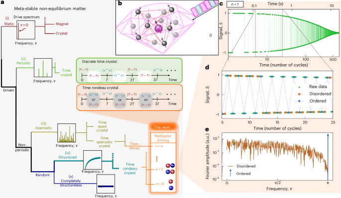
Higher-order multipolar operators of order n can be recursively constructed as \({U}_{n}^{\pm }={U}_{n-1}^{\mp }{U}_{n-1}^{\pm }\) by anti-aligning (n − 1)-multipole pairs together. The length of an n-multipole sequence grows exponentially in n as 2nT. In complete analogy, the n-RMD protocol consists of the sequential application of a random selection of \({U}_{n}^{\pm }\) with equal probability. In the limit n→∞, the protocol becomes deterministic and aperiodic in time. It indeed corresponds to the Thue–Morse sequence, which has also been extensively studied in the context of, for instance, quasicrystals and number theory37,53.
Prethermal order
Generic time-dependent many-body systems do not obey the energy conservation law. Therefore, they tend to absorb energy from the external drive, and eventually heat up towards a featureless state at infinite temperature. Although in generic closed systems, Floquet heating cannot be avoided entirely, it can be significantly suppressed if there is a notable mismatch between the local energy scale and the external driving frequency, for instance, in the high-frequency regime54. This can result in an exceptionally long-lived prethermal regime before notable heating happens55,56,57,58. Within this regime, dynamics can be approximated by a static quasiconserved effective Hamiltonian Heff, which can be perturbatively constructed, for instance, by using a Floquet–Magnus expansion or high-frequency expansion59,60. To avoid the eventual heat death of periodically driven systems entirely, non-ergodic, periodically driven many-body localized systems need to be considered10,24; however, their experimental realization—requiring strongly disordered one-dimensional systems61,62—is challenging in practice.
For ergodic interacting many-body systems, the existence of the effective Hamiltonian implies that during the prethermal regime, the local properties of the system can be captured by a prethermal canonical ensemble \({\rho }_{{\rm{pre}}} \approx {\rm{e}}^{-{\beta }_{{\rm{eff}}}{H}_{{\rm{eff}}}}\); here βeff denotes the prethermal temperature that is determined by the energy density of the initial state56. If βeff is sufficiently low and Heff allows for spontaneous symmetry breaking to occur at a finite temperature, ρpre can exhibit equilibrium spatial ordering. Additionally, if regular polarization inversion is further introduced by the drive, as described in the ‘Non-periodic deterministic drives: aperiodic and quasiperiodic sequences’ section, prethermal non-equilibrium time-crystalline order can form63,64.
This prethermal phenomenon can be generalized to other time-dependent protocols even in the absence of strict temporal periodicity. One typical example is quasiperiodically driven systems in which at least two drive frequencies are incommensurate with each other26,27,28,29,65,66,67,68,69. Prethermalization also occurs in RMD systems, where the driving spectrum has continuous support over the entire range of frequencies due to temporal randomness70.
The temporal multipolar correlation of RMD protocols significantly modifies the Fourier spectrum of the random drive sequence: ref. 70 shows that the envelope of the spectrum follows \(\mathop{\prod }\nolimits_{j = 1}^{n}{[1-\cos \left({2}^{j-1}\nu \right)]}^{1/2}\), where ν is the Fourier frequency. This expression indicates an algebraic suppression νn for ν→0. Since it is these low-frequency modes that normally produce the dominant contribution to heating, heating can be algebraically suppressed in the high-frequency regime. The algebraic scaling exponent also has an explicit dependence on multipolar order. One can also construct effective Hamiltonians by generalizing the Floquet–Magnus expansion and use the linear response theory to analyse the heating behaviour more systematically39. Let us emphasize that although prethermalization is readily extended beyond Floquet systems, to the best of our knowledge, the suppression of heating in many-body localized systems driven with random structured drives has not been demonstrated so far. Investigating possible routes to avoid heating in random structured drives is an interesting question for future work, and would open the possibility for an absolutely stable rondeau phase of matter and further tools to investigate them71,72,73.
If the temporal randomness only weakly perturbs the system, the RMD protocol indeed leads to a prethermal plateau, which can feature either equilibrium or non-equilibrium ordering, very similar to Floquet systems. However, the RMD protocol introduced in the ‘Non-periodic deterministic drives: aperiodic and quasiperiodic sequences’ section is designed such that temporal randomness in polarization inversion strongly changes the behaviour of micromotion of the system. As illustrated in the main text, this RMD protocol results in a rondeau order, beyond the conventional Floquet paradigm.
It is worth noting that although those prethermal orders eventually melt, their stability and lifetime can be parametrically controlled, permitting direct experimental observation with our current nuclear spin setup. Throughout, we estimate the lifetime via the 1/e decay time Te defined as the time in which the absolute value of the signal is closest to 1/e of its initial value S0, that is,
$${T}_{e}={\rm{argmin}}t > 0\,| | S(t)| -{S}_{0}/e| \,.$$
(3)
This feature may also be exploited to study interesting applications (see the main text).
DFT
In the main text, we use two different DFTs. For micromotion, we consider the DFT of the digitized micromotion extracted at times (2ℓ + 1)T/2 (\(\ell \in {\mathbb{N}}\)):
$${{\rm{DFT}}}_{{\rm{micro}}}({\nu }_{k})=\frac{1}{M}\mathop{\sum }\limits_{\ell =0}^{M-1}{\rm{e}}^{-{\rm{i}}{\nu }_{k}\ell }{\rm{sgn}}\left(S((2\ell +1)T/2)\right)\,,$$
(4)
where νk = k2π/M, k = 0…M − 1 and sgn(S(t)) = +1 or sgn(S(t)) = –1 depending on whether S(t) > 0 or S(t) < 0, respectively. Note that \(t=(\ell +\frac{1}{2})T\) was chosen for convenience, any other times t = ℓT + t0 with t0 such that the \(\hat{{\bf{y}}}\) pulse has already occurred for ⊕ but not for ⊖, that is, N+τ < t0 < N−τ; note also that this ‘disordered’ regime depends on the choice of N±, which are adjustable experimental parameters.
For the stroboscopic evolution, we consider the DFT of the signal extracted at stroboscopic times ℓT (\(\ell \in {\mathbb{N}}\)):
$${{\rm{DFT}}}_{{\rm{strobo}}}({\nu }_{k})=\frac{1}{M}\mathop{\sum }\limits_{\ell =0}^{M-1}{{\rm{e}}}^{-{\rm{i}}{\nu }_{k}\ell }S(\ell T)\,;$$
(5)
similarly, times \(t=\ell T+{t}_{0}^{{\prime} }\) with \({t}_{0}^{{\prime} } < {N}_{+}\tau\) or \({t}_{0}^{{\prime} } > {N}_{-}\tau\) are also possible. Note that the Fourier amplitude is defined as the absolute value of the DFT (Fourier amplitude = ∣DFT∣), in contrast to the Fourier intensity (that is, the power spectrum), which is defined as the absolute value squared.
Classification of drives and their Fourier transformsInteger representation and DFT
A similar DFT can be defined for the RMD drives considered in the main text. Specifically, all RMD drives can be described as an ordered sequence of ⊕ and ⊖ (Fig. 2); therefore, by identifying ⊕ and ⊖ with numbers +1 and –1, respectively, any drive instance is uniquely determined by a sequence \({\mathcal{S}}={s}_{n}\), n = 1, 2…sn ∈ {+1, –1} (for example, Extended Data Fig. 1, top). Instead, we consider the DFT of the drive sequence given by
$${{\rm{DFT}}}_{{\rm{drive}}}({\nu }_{k})=\frac{1}{M}\mathop{\sum }\limits_{\ell =0}^{M-1}{{\rm{e}}}^{-{\rm{i}}{\nu }_{k}\ell }{s}_{\ell }\,,$$
(6)
where νk = k2π/M, k = 0…M − 1. In analogy to the signal DFTs, the Fourier amplitude is defined as the absolute value of the DFT; this definition of the drive Fourier amplitude, using the integer representation of the drive, is used in Fig. 3.
Note that this DFT should not be confused with the continuous Fourier spectrum of its generating drive, which is sketched in Fig. 1a. In particular, by assigning integers to the ⊕/⊖ sequences, we coarse-grain over the details of the monopoles. This results in a loss of information that can alter the resulting discrete Fourier spectrum. For instance, the Floquet sequence (+1, +1, +1…) has a DFT that is indistinguishable from that of a static (time-independent) drive, and the n = 0 sequence (for example, (+1, –1, –1, –1, +1, +1, –1…)) has an entirely flat spectrum, suggesting that this drive corresponds to a completely structureless drive; however, both these observations are wrong since the inner structure of the ⊕/⊖ are ignored: the Floquet sequence is a periodic time-dependent sequence since the \(\hat{{\bf{y}}}\) pulses within one ⊕/⊖ are not always on, and the n = 0 sequence is structured because only one of two structured sequences is applied.
Continuous Fourier transform
To restore the entire information of the drives, the Fourier transform of the analogue drive should be considered, which we refer to as continuous Fourier transform. In our case, the drive relevant for the temporal order is the \(\hat{{\bf{y}}}\) field; more generally, we can consider an arbitrary driving field, d(t), that couples to the system and can induce temporal order: H(t) = H0 + d(t)V. In Extended Data Fig. 1, we display the analogue drives and the corresponding continuous Fourier spectra for some of sequences considered in this work, where, for simplicity, we consider \(\hat{{\bf{y}}}\) to follow a square pulse. The different drives display the distinct features sketched in Fig. 1a(ii)–(iv); to obtain the two missing features (i) and (v), a constant drive d(t) = d and completely random drive d(t) = ξt, with white noise \({\mathbb{E}}({\xi }_{t})=0\) and \({\mathbb{E}}({\xi }_{t}{\xi }_{{t}^{{\prime} }})=\delta (t-{t}^{{\prime} })\cdot {\rm{const}}\) (where \({\mathbb{E}}\) denotes the expectation value), can be used, respectively. However, neither of these two realizes a stable temporal order.
Non-periodic deterministic drives: aperiodic and quasiperiodic sequences
In the phylogenetic tree of drives (Fig. 1a), we reported on the experimental observation of a time aperiodic crystal arising from the Thue–Morse sequence. Here, for completeness, we also report on the experimental observation of a time quasicrystal using the famous Fibonacci sequence (Extended Data Fig. 2). The Fibonacci sequence is defined via the recursive relation (n ≥ 2)
$${U}_{n}={U}_{n-2}{U}_{n-1}\,,$$
(7)
which is initialized by the elementary building blocks U1 = ⊕ and U0 = ⊖.
Quasiperiodic drives form a special subclass of aperiodic drives, which can be characterized by a finite number of incommensurate frequencies. Hence, their Fourier spectra consists of only finitely many independent frequencies ν1…νk (k < ∞) and integer linear combinations of these, that is, P(ν) ≠ 0 only if \(\nu =\mathop{\sum }\nolimits_{j=1}^{k}{\ell }_{j}{\nu }_{j}\), where \({\ell }_{j}\in {\mathbb{Z}}\). Although there have been various numerical and analytical studies on the heating properties of specific aperiodic39 and quasiperiodic28 drives, as of now, a systematic classification of the heating property in generic aperiodically driven many-body systems is missing.