
Description of historical trends in cryptocurrencies and NFT market
Figure 1a and Fig. 1b depict the historical prices of Bitcoin and Ethereum respectively. Based on the figures, the prices of Bitcoin and Ethereum underwent a rapid surge starting in 2020 and continuing until early 2021. To be more specific, Bitcoin reached its relatively high price levels earlier and sustained them for a longer period, fluctuating within the upper price range during the first quarter of 2021, whereas Ethereum’s price only reached a relatively high level during the first month of the second quarter, and its duration was very short. Subsequently, the prices dropped substantially until July, marking a nearly 50% decrease from their peak levels. The prices then rebounded in the following two months, reaching a second peak in September 2021. However, from that point onwards, the prices experienced a steep decline, ultimately plummeting by a staggering 77% by 2023.
Fig. 1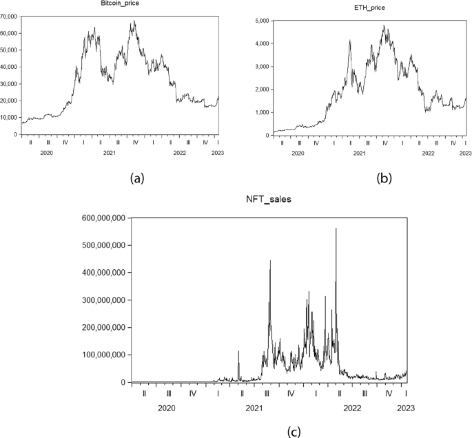
a Historical price of Bitcoin (b) Historical price of Ethereum (c): Historical NFT Sales Volume (in USD).
Figure 1c presents the historical sales volume of the NFT market. Based on the figure, the sales volume remained relatively low in 2020, gradually increased in early 2021, and experienced a significant surge in May. Throughout 2021, NFT sales volume exhibited rapid growth and substantial fluctuations, with sales increasing nearly 100 times compared to 2020. Notably, August 2021 witnessed an incredible surge in NFT sales volume, while the remaining months of 2021 experienced a decline. However, as we may note from Fig. 1c, starting from the first quarter of 2022, the sales volume increased and fluctuated. In April 2022, the sales volume reached its peak. Conversely, after May 2022, the sales volume experienced a significant decline, reaching a lower level, although it remained higher than the sales record in 2020.
Market herding behavior analysis
Figure 2a, b present the time-varying herding behavior observed in the cryptocurrency market and the NFT market, respectively. The analysis utilizes a rolling window method with a length of 14 days, selected to effectively capture the underlying trends. In these figures, if the t-statistics fall below the negative 10% critical value line (indicating that negative γ2 becomes statistically significant), it indicates the presence of herding behavior.
Fig. 2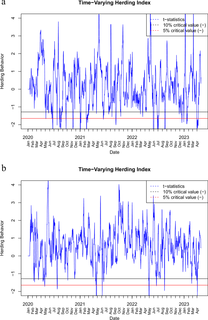
a Time-varying Herding in the Cryptocurrency Market. b Time-varying Herding in the NFT market. In these figures, if the t-statistics fall below the negative 10% critical value line (indicating that negative \(\gamma 2\) becomes statistically significant), it indicates the presence of herding behavior.
From May 2020 to the beginning of 2021, the cryptocurrency market experienced multiple herding periods, as shown in Fig. 2(a). These periods could be attributed to macroeconomic uncertainty and the rapid growth of the cryptocurrency market. According to Sharma (2021), uncontrolled economic stimulus measures implemented during the economic slowdown, such as extensive money printing coupled with macroeconomic instability resulting from low-interest rates, led to the depreciation of the dollar, increased inflation rates, and raised investor concerns. However, the halving of Bitcoin in May 2020, which reduces the rate of Bitcoin inflation and emphasizes its scarcity, encouraged investors to shift their funds from dollars to cryptocurrencies (Copeland, 2020). In late 2020, the announcement of investments in cryptocurrencies and their trading ecosystems by institutional investors and banks had a significant impact, particularly benefiting Bitcoin and fueling investor frenzy (Sharma, 2021). These factors contributed to the herding behavior observed during this period in the cryptocurrency market as depicted in Fig. 2(a).
In 2021, the herding behavior observed in the cryptocurrency market aligns with a period characterized by cryptocurrency price volatility, often referred to as a bubble period. During this period, significant price fluctuations were witnessed in Bitcoin. For instance, from February to March, the price of Bitcoin surged to new highs before experiencing a minor decline. Subsequently, following a bottoming out in July, Bitcoin and other cryptocurrencies embarked on a solid recovery, partially driven by Elon Musk’s engagement with leading Bitcoin mining companies to develop more sustainable and efficient mining practices (Ante, 2023). These specific timeframes in 2021 coincide with the bubble period, providing evidence of time-varying herding behavior in traditional cryptocurrencies. The herding behavior observed during this period reflects market participants’ responses to the price volatility and rapid changes in the cryptocurrency market.
It is interesting to note that in 2022, the herding behaviors observed in the cryptocurrency market, as shown in Fig. 2a, coincided with the Federal Reserve’s announcements of interest rate increases. This suggests that investor herding behavior is influenced by economic policy, which aligns with the conclusions drawn by Omane-Adjepong et al. (2021). Bitcoin, as the most prominent cryptocurrency, is often perceived as a hedge against risks associated with traditional currencies, such as the dollar. This perception is evident from the investor herding behavior observed in both 2020 and 2022. According to Corbet et al. (2019), monetary policy decisions made by the FOMC, particularly those concerning interest rates, exert a significant impact on Bitcoin prices. The herding behavior observed in 2020 can be attributed to low-interest rates and macroeconomic uncertainty, leading to a surge in cryptocurrency prices, as depicted in Fig. 1a, b. Conversely, as investors perceive the dollar as a stable currency with minimal risk of rapid depreciation, the Federal Reserve’s decision to raise interest rates by 25 basis points in March, followed by an additional 50 basis points in May, culminating in a 75-basis point increase in June 2022, becomes even more appealing (see Table 2, Panel B). This prompts investors to shift their funds from risky cryptocurrency investments to dollar-denominated financial markets, resulting in a significant decline in cryptocurrency prices.
Table 2 Description of Major Events Influencing Herding Behavior.
These findings consequently imply the potential utility of Bitcoin as a risk management tool, particularly in the face of unpredictable interest-rate risk shocks. They suggest that investors may consider incorporating Bitcoin into their portfolios as part of their risk analysis and management strategies.
To further analyze the linkage between events and herding behaviors, Table 2 shows the major event announcements related to the dates when herding behavior is observed. According to Table 2, Panel A, herding behavior occurs from 3 days before to 10 days after the announcement, except for the event on July 21, 2021. The herding behavior related to “The B Word” conference begins 10 days prior to the event, as the press had forecasted and informed the public in advance. Moreover, herding behavior is not persistent over time but it occurs periodically. Specifically, herding behaviors are observed prior to the announcement date; however, the public tends to appear calm as the actual event date approaches, including on the announcement date itself. After the announcement, the public’s response can be either immediate or delayed, depending on whether the announcement meets their expectations. This is in line with the observation by Qiang (2023).
Table 2b presents the relationship between the Federal Open Market Committee (FOMC) meeting dates and the herding dates during 2022 and 2023. Investors tend to respond to the announcement more quickly than they do to a 50 bp hike, while no herding behavior is observed in response to a 25 bp hike except on March 22, 2023. The main reason for the herding behavior observed is attributed to the failure of Silicon Valley Bank (SVB) (Jin and Tian, 2024). Moreover, investors postponed their reaction during the herding period on October 12th, primarily because Bitcoin’s value increased further as global markets improved, and traders were awaiting the release of US Consumer Price Index (CPI) data while also monitoring a significant upgrade to the Ether blockchain (Bloomberg, 2022; Qiang, 2023). The herding behavior predominantly occurred prior to the announcement, driven by investors’ expectations.
Figure 2(b) specifically illustrates the presence of herding behavior in the NFT market, as evidenced by the consistently falling time-varying t-statistics below the critical value line. From February to August 2020, the presence of herding behavior in the NFT market can be attributed to market inefficiencies, aligning with the findings of Bao et al. (2022) and Dowling (2022a). The year 2021 witnessed the rise of NFTs, marked by a significant surge in NFT sales volumes occurring in May 2021, as depicted in Fig. 1(c). This surge in activity explains the occurrence of herding behavior during that period as depicted in Fig. 2(b). Furthermore, herding behavior can be observed in the NFT market from May to September 2022 and April 2023. Concurrently, the cryptocurrency market also exhibits herding behavior (see both Figs. 2a, b). Thus, our hypotheses H1 and H2 are both supported. Consequently, it is reasonable to speculate that there may be a causal relationship between the NFT and cryptocurrency markets.
Relationship between cryptocurrency and NFT markets
Table 3 presents the descriptive statistics for the variables under study. It is observed that all variables have mean values greater than their corresponding standard deviations, indicating an under-dispersed distribution. Additionally, the Jarque and Bera (1987) test results indicate that none of the variables follow a normal distribution. This suggests that Bitcoin prices, Ethereum prices, sales volume, and the number of unique buyers in the NFT market exhibit volatility and instability throughout the selected period.
Table 3 Descriptive statistics.
Unit root test results (Augmented Dickey-Fuller (ADF)) are shown in Table 4, indicating that all the variables are stationary at their first difference level, which means that they are in the same order of integration, making VAR a suitable method. Yet, as shown in Table 5, on the basis of eigenvalues, Trace test and Maximum Eigenvalue test, our Johansen test of cointegration indicates one cointegration relationship, thus making the VECM as our model. Based on the AIC, we adopt the model with lag seven, following the approach of Ante (2022a) and Apostu et al (2022), to examine the linkage between the NFT and cryptocurrency markets.
Table 5 Johansen cointegration test.
After confirming the presence of a long-run association between our variables, we examine the long-run dynamics among these variables. Before establishing the VECM, we check for the presence of serial correlation in our model with the Lagrange Multiplier (LM) test. The results show that all the p-values (in Table 6) are greater than 5%, suggesting that there is no evidence of serial correlation in our model.
Table 6 VEC Residual Serial Correlation LM Tests.
The results of our VECM indicate a negative and significant sign of the error correction term, which implies the existence of a long-run relationship among the proposed variables. The long-run relationship among the proposed variables for one cointegrating vector is displayed below (standard errors are displayed in parenthesis).
$$\begin{array}{l}{{ect}}_{t-1}=1.00\Delta {{\rm{In}}\;{\_}{{sales}}}_{t-1}-0.46\Delta{{\rm{In}}\;{\_}{eth}}_{t-1}-1.17\Delta{{\rm{In}}\;{\_}{buyer}}_{t-1}\\\qquad\quad\;\;\;-\,0.82\Delta{{\rm{In}}\;{\_}{btc}}_{t-1}+5.47(0.46)(-0.11)(-0.41)\end{array}$$
(6)
$$\begin{array}{l}\Delta {\rm{In}}\;{\_}{{sales}}_{t}=-0.1429{{ect}}_{t-1}-0.3300\Delta {\mathrm{ln}}\;{\_}{sales}_{t-1}+\ldots\\\qquad\qquad\qquad\;+\,0.0101+0.0378{herding}(-0.03)\end{array}$$
(7)
In the following analysis, we present the Granger Causality Test results to interpret the VECM findings. Table 7 displays the short-run Granger causality test results, which assess whether a change in one variable precedes a change in other variables. These statistics are computed for each combination of our dependent and independent variables.
Table 7 Granger causality test results based on VECM.
To illustrate, the first row of results shows whether all independent variables (ETH price, the number of unique buyers and Bitcoin price) significantly impact NFT sales. Since the estimates of these independent variables exceed the significance threshold of 10%, we cannot conclude that ETH price, Bitcoin price, and the number of unique buyers Granger-cause NFT sales. The third row shows the relationship between the number of unique buyers and the other variables. It demonstrates similar results, indicating that neither Bitcoin price, Ethereum price, nor NFT sales Granger cause the number of unique buyers. However, the second and fourth rows of results reveal that, there is a Granger-causal relationship between the price of Bitcoin and the price of Ethereum. Additionally, the number of unique buyers Granger causes the prices of both cryptocurrencies. The causality results remain unaltered with the herding dummy incorporated into the model.
Based on the Granger Causality Test results, we conclude that the prices of cryptocurrencies have a mutual influence on each other including during the period of cryptocurrency market herding, but the herding effect does not spill over into the NFT market. However, the number of investors participating in the NFT market can have an impact on the prices of cryptocurrencies, namely the prices of Bitcoin and Ethereum.
Robustness testRobustness check with alternative variables
We conduct a further test by substituting variables. Specifically, we replace the number of unique buyers in the NFT market with the number of unique sellers. It is important to note that variables in the further test are stationary at I(1), and again the Johansen cointegration test confirms the existence of a long-term equilibrium relationship between them.
Table 8 presents the results of our robustness test, which reveal important insights. The number of unique sellers exhibits a Granger-causal relationship with NFT sales volume at the 1% significance level (see first row of Table 8). Conversely, NFT sales volume Granger-causes the number of unique sellers at the 10% significance level, as indicated in the third row. However, the null hypothesis that the prices of cryptocurrencies (Bitcoin and Ethereum) do not Granger-cause NFT market-related variables is accepted (see first and third rows of Table 8). Moreover, the price of Ethereum is influenced by both the number of unique sellers in the NFT market and the price of Bitcoin (see second row of Table 8). Combined with the result mentioned above, where the number of unique buyers Granger-causes Ethereum’s price, this enhances our findings that investors in the NFT market have a significant impact on Ethereum’s price. On the other hand, Bitcoin’s price is influenced by Ethereum’s price at the 5% significance level, indicating a Granger-causal relationship between these two cryptocurrencies during periods of market herding. However, NFT market-related variables do not significantly affect Bitcoin’s price (see forth row of Table 8). Based on these results, we can infer that the NFT market may impact the cryptocurrency market by influencing the price of Ethereum. This suggests that changes and activities in the NFT market can potentially influence the dynamics of the broader cryptocurrency market. Thus, hypothesis H3 is supported.
Table 8 Robustness Test for Granger Causality.Robustness check with impulse response functions
Our Granger causality results suggest that, the number of investors in the NFT market have cross-market influence in cryptocurrencies’ prices. To further analyze the dynamic mutual effects of cryptocurrency prices and the number of investors in the NFT market in the short run, impulse response functions are employed. Figure 3 shows the relevant impulse response function results. Specifically, it illustrates the response of cryptocurrency prices to a unit shock in the number of investors, including both unique sellers and buyers, and also shows the response of investors to a unit shock in cryptocurrencies prices.
Fig. 3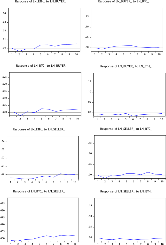
Impulse response functions. Impulse response functions based on the VECM are shown for a time horizon of ten days.
Unlike VAR, impulse response functions of a VECM need not return to their mean value, as series are cointegrated in the long-run (Mills, 1998, Ante, 2022b). During the initial two periods, the response of cryptocurrency prices (as shown by the four diagrams in the left column of Fig. 3) to a unit shock in the number of investors (both unique buyers and unique sellers) in the NFT market is negative and exhibits a decreasing trend. Following slight fluctuations in the 3rd and 4th periods, there is a sharp increase in the response of cryptocurrency prices from the 5th period onwards that can be considered significant. However, as shown by the four diagrams in the right column of Fig. 3, the number of investors shows slight changes in response to the shock of cryptocurrencies and converges to zero as the effects of the shock die out. Comparing the left and right columns of Fig. 3, we observe that the shock from the number of investors lasts longer on cryptocurrency prices as expected. This indicates that the number of investors Granger-causes the prices of cryptocurrencies in the long run. In addition, long-term herding effects captured by the VECM model reflect more stable, equilibrium-driven behaviors that emerge over extended periods. The unique buyer would cause the increasing price of cryptocurrencies for both Bitcoin and Ethereum; however, the increasing price of cryptocurrencies would not cause an increase in the number of unique active wallets (both sellers and buyers) in NFT markets.
Overall, impulse response functions are helpful in mapping the short-run effects and thus complementing the results of the Granger causality tests. Specifically, the results show that the shock from the number of NFT investors (both buyers and sellers) on cryptocurrency prices lasts longer as expected, while the response of the number of investors in the short-run equilibrium adjustment process is rather fast.