
Dynamic mean-field model
In this work, we use the DMF model proposed in prior work21 to simulate the brain dynamics. It describes the dynamics of the network containing excitatory and inhibitory populations of spiking neurons interconnected via NMDA synapses. The global brain dynamics of the interconnected local networks can be expressed by the following nonlinear differential equations:
$$\left\{\begin{array}{l}\dot{{S}_{i}}=-\frac{{S}_{i}}{{\tau }_{S}}+r(1-{S}_{i})H({x}_{i})+\sigma {\xi }_{i}(t)\quad \\ {x}_{i}=wJ{S}_{i}+GJ{{{\Sigma }}}_{j}{C}_{ij}{S}_{j}+{I}_{0}\hfill \\ H({x}_{i})=\frac{a{x}_{i}-b}{1-\exp (-d(a{x}_{i}-b))}\hfill \end{array}\right.$$
(1)
where Si denotes the average synaptic gating variable at the ith local cortical area, which is the state variable with time dependency; xi and H(xi) are intermediate variables denoting the total input current and the population firing rate at the ith area, respectively. The range of i varies along with the number of areas in the dataset. The local excitatory recurrence w, the external input I0, and the global scaling factor of information strength G are the parameters we need to tune through model inversion. Cij denotes the structural connectivity (SC) between the ith and the jth areas, which can be derived from dMRI data. ξi(t) corresponds to the Gaussian noise in the dynamic system, and σ is the amplitude, which can also be tuned. Here, we fix σ to 0.001 for simplicity since it typically falls around the value after identification. The other variables in the equations are all constant parameters. The value of synaptic coupling J is set to be 0.2609 (nA). The parameter values for the input-output functions H(xi) are a = 270(n/C), b = 108(Hz), and d = 0.154(s). The kinetic parameters for synaptic activity are r = 0.641 and τS = 0.1(s).
To identify the DMF model with empirical data, we need to simulate the blood-oxygen-level-dependent (BOLD) fMRI signals further with the Balloon-Windkessel hemodynamic model87. The dynamic process linking synaptic activities to BOLD signals is governed by
$$\left\{\begin{array}{l}\dot{{z}_{i}}={S}_{i}-\kappa {z}_{i}-\gamma (\; {f}_{i}-1)\hfill \\ \dot{{f}_{i}}={z}_{i}\hfill \\ \tau \dot{{v}_{i}}={f}_{i}-{v}_{i}^{1/\alpha }\hfill \\ \tau \dot{{q}_{i}}={\frac{{f}_{i}}{\rho }}[1-{(1-\rho )}^{1/{f}_{i}}]-{q}_{i}{v}_{i}^{1/\alpha -1}\quad \end{array}\right.$$
(2)
where Si is the same variable as in the DMF model. The vasodilatory signal zi, the inflow fi, the blood volume vi, and the deoxyhemoglobin content qi are four state variables. The BOLD signal follows
$${{BOL{D}}}_{i}={V}_{0}[{k}_{1}(1-{q}_{i})+{k}_{2}(1-\frac{{q}_{i}}{{v}_{i}})+{k}_{3}(1-{v}_{i})].$$
(3)
The principles of the model and parameter values can be found in prior work87, and are not repeated here. Combining DMF and the hemodynamic model, we can simulate the brain activity as well as the BOLD signals, which can also be measured using fMRI empirically.
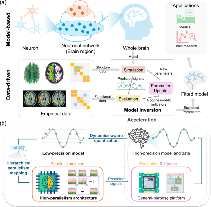
Semi-dynamic quantization for brain dynamics
The commonly used data types on intelligent computing platforms can be divided into two categories: floating-point types and integer types. GPUs usually possess large capacities for floating-point computing, supporting full-precision formats like Float32 (FP32) and half-precision formats like Float16 (FP16) or BFloat16 (BF16). Implementing dynamical models with these data types is not difficult because their range and precision are sufficient to represent the model variables in most cases. In contrast, the most popular low-precision integer formats in brain-inspired computing chips are signed 8-bit integers (INT8) and unsigned 8-bit integers (UINT8), both of which are limited to 256 distinct values. Here, we introduce the approach to simulate brain activities using the integer format.
The mapping of values from a continuous set to a countable, smaller set is called quantization in the signal processing and AI domains. The principle of uniform quantization can be written as
$$x\approx \hat{x}=s({x}_{{{{\rm{int}}}}}-z),$$
(4)
where x and xint are the original real-valued variable and the quantized variable, respectively. \(\hat{x}\) is the approximate value represented by the low-precision data. The quantization is primarily a simple affine transformation with two parameters, namely the scaling factor s and the zero point z. Thus, the quantization function is defined as
$${x}_{{{{\rm{int}}}}}={{{\rm{clamp}}}}(\lceil \frac{x}{s}\rfloor+z;{q}_{\min },{q}_{\max })$$
(5)
where ⌈ ⋅ ⌋ corresponds to the round function. The equation rounds the scaled real-valued variable to an integer and then clamps it to the range of the integer format (\([{q}_{\min },{q}_{\max }]\)).
We use semi-dynamic quantization to determine the scaling factor s and zero point z for both the DMF model and the hemodynamic model. During the warm-up stage, the model quickly converges near the fixed point. Then we determine the quantization parameters based on the variable ranges in the QPS stage. We can calculate the power-of-two scaling factor for each of them using
$$\left\{\begin{array}{l}{s}_{{{{\bf{y}}}}}={2}^{-\lfloor {\log }_{2}({q}_{\max }/{y}_{m})\rfloor }\hfill \\ {y}_{m}=\left\{\begin{array}{ll}\max (| {{{\bf{y}}}}| )\quad &{{{\rm{symmetric}}}}\,{{{\rm{quantization}}}}\\ \frac{\max ({{{\bf{y}}}})-\min ({{{\bf{y}}}})}{2}\quad &{{{\rm{asymmetric}}}}\,{{{\rm{quantization}}}}\end{array}\right.\quad \end{array}\right.$$
(6)
where ⌊ ⋅ ⌋ represents the floor function, and ∣ ⋅ ∣ represents the absolute value. qmax is the maximum positive value of the signed integer type, and it is 127 for INT8 here. The bold y is the variable that needs to be quantized. As most brain-inspired computing chips only support per-tensor quantization, we treat the same variable within each node of a model as a vector and apply uniform quantization parameters to all elements in it. Thus, the shape of y here is (N, TQPS), where N denotes the number of nodes in a model and TQPS is the number of time steps in the QPS stage. ym represents the unilateral maximum range that needs to be expressed by the integer type, which can be obtained using the extreme values of the vector in the QPS stage. Similarly, the zero point z can also be calculated by
$${z}_{{{{\bf{y}}}}}=\left\{\begin{array}{ll}0\hfill &{{{\rm{symmetric}}}}\,{{{\rm{quantization}}}},\\ \frac{\max ({{{\bf{y}}}})+\min ({{{\bf{y}}}})}{2}\quad &{{{\rm{asymmetric}}}}\,{{{\rm{quantization}}}}.\end{array}\right.$$
(7)
In the subsequent simulation stage, all variables are represented as integers. We can envision scenarios where the ranges of variables change significantly during model execution. If such changes are predictable, semi-dynamic quantization could still be employed. For instance, when simulating brain lesions88, perturbations are typically introduced to a baseline resting-state brain model. These perturbations can cause the model to transfer from one stable state to another. Since the timing of these perturbations is known as a priori, high-precision floating-point numbers could be used for the transition phase, while a new low-precision quantization scheme could be employed once another stable state is reached. By iteratively applying the warm-up and simulation stages, the semi-dynamic quantization method could be potentially extended to more complex scenarios.
Influences of range-based group-wise quantization
We propose a range-based group-wise quantization method to address the spatial heterogeneity of the hemodynamic model. Figure 2b shows that some variables exhibit a multimodal distribution across the whole-brain model, where the values from different brain regions tend to cluster within several distinct ranges. The most straightforward way to reduce quantization errors from using a single set of parameters across brain regions is to group regions by distribution peaks and calculate parameters for each group separately. However, the variable distributions vary significantly across different empirical data and model parameters, leading to unstable results with inconsistent numbers of groups and varying group sizes. Therefore, we adopt a simpler grouping method: we evenly divide the entire range of variables across the whole-brain model into multiple intervals and sequentially group the regions whose maximum variable values fall within the same interval, from the lowest to the highest. The number of groups (i.e., the number of intervals) can be determined based on the model size (i.e., the number of brain regions), preventing excessive computational overhead from too many groups.
We apply such a range-based group-wise quantization method to three variables in the hemodynamic model: the blood flow f, the blood volume v, and the deoxyhemoglobin content q, as they exhibit the most pronounced spatial heterogeneity. In Supplementary Fig. S3a, we show the goodness-of-fit indicators obtained from simulations at the same sampling points as in Fig. 3a, using low-precision models without group-wise quantization. The distributions are close to those from the high-precision models and the low-precision models with group-wise quantization in Fig. 3a. We further test the distribution of three indicators along a line in the parameter space using different models. The low-precision models without group-wise quantization show satisfactory results in FC correlation and metastability, differing from their group-wise quantized counterparts mainly in slightly lower indicator values and increased G-dependent fluctuations. However, they are almost unusable if we measure the similarity between simulated and empirical functional connectivity dynamics (FCD) matrices by calculating the Kolmogorov–Smirnov (KS) distance between their probability distribution functions (pdfs). This demonstrates that group-wise quantization significantly aids low-precision models in reproducing the spatiotemporal dynamics of the brain network. Nevertheless, since model inversion does not require all indicators for parameter evaluation, we believe that low-precision models without group-wise quantization still retain a certain practical value.
Determining the time steps for multi-timescale simulation
The state variables within a dynamic system may fluctuate on different timescales temporally. The brain dynamics model serves as a good example of such temporal heterogeneity. As demonstrated in Supplementary Fig. S1, some state variables (f, v, and q in the hemodynamic model) exhibit much slower temporal dynamics compared to the others such as S in the DMF model and z in the hemodynamic model. In other words, the difference in some variables between two adjacent time steps (Δx[t]) is smaller. Therefore, it is necessary to use a smaller scaling factor (\(\frac{\Delta x}{s} > 1\)) to distinguish consecutive values of such “slower” variables (x[t] and x[t + 1] = x[t] + Δx[t]). However, as aforementioned, a smaller scaling factor will also sacrifice the representation range of the integer, resulting in substantial truncation errors. To resolve this dilemma, we increase the simulation time step size Δt for the simulation because a larger Δt may lead to a larger temporal difference Δx with the same differential equation, which may relax the requirement for the scaling factor s. Meanwhile, a larger time step can also reduce the number of iterations needed for a given simulation time, thus accelerating the entire simulation process.
However, this does not address all challenges, as another dilemma emerges in the selection of the time step size: if only the “slower” variables are considered and a large time step is used for all variables, it may affect the accuracy of the Euler integration; while if a smaller time step is employed, we will again encounter the scaling factor problem where the “slower” variables cannot be correctly quantized to lower precision. Supplementary Fig. S1 shows the simulated brain dynamics signals using different global time step sizes. When using the same time step as the high-precision simulation (e.g., 0.01 s), the “slower” variables show such small temporal variations that they cannot be represented by integers, resulting in quantized variables remaining constant over time (issue A). When the time step is increased to 0.18 s, z exhibits normal temporal evolution, but the variables f, v, and q still show periods of constant values, with the “slowest” q being notably more affected than f and v (issue B). As the time step further increases (e.g., 0.36 s and 0.54 s), while all variables no longer show significant value stagnation, the oscillation amplitudes of the “faster” variable (z) significantly exceed those of the high-precision model, indicating stability issues in the dynamical model due to excessive time steps (issues C and D). Overall, it is difficult to find a single global time step that meets the requirements of all variables.
In fact, for a state variable x with a time derivative \({\dot{x}}\), the low-precision simulation is constrained by
$$\frac{{x}_{{{{\rm{range}}}}}}{{\min }_{{\dot{x}}\ne 0}| {\dot{x}}| }\le {2}^{b-1}\Delta t$$
(8)
where \({\min }_{{\dot{x}}\ne 0}| {\dot{x}}|\) denotes the minimum effective absolute value (i.e., the smallest absolute value that needs to be distinguished from zero) of the time derivative, xrange is the maximum unilateral range that must be represented for variable x when quantized to lower precision, b represents the bitwidth of the low-precision integer, and Δt is the simulation time step size. Note that \({\min }_{{\dot{x}}\ne 0}| {\dot{x}}| \Delta t\) represents the minimum effective change in this variable, which needs to be represented by integer 1 in the low-precision simulation; while xrange needs to be represented by the maximum integer value (2b−1). Therefore, this equation implies that both ranges of the variable and its time derivative must fit into the integer representation, establishing a lower bound for the simulation time step size. It merits clarification that both xrange and \({\min }_{{\dot{x}}\ne 0}| {\dot{x}}|\) are not necessary to be the actual bounds of the high-precision values, as the quantization process tolerates certain levels of rounding and truncation errors. We visualize the relationship between the variable ranges and the time derivatives in Supplementary Fig. S2. The distributions of the variables and their absolute time derivatives are shown in Supplementary Fig. S2a. We calculate a temporal scale index τ by using \(({x}_{\max }-{x}_{\min })/2\) to represent the range of the variable x and characterizing its minimum effective non-zero absolute derivative value with the first quartile. From the indices in Supplementary Fig. S2b, we can observe that z requires a much larger simulation time step size compared to S, f, and v demand larger time step sizes over z, and q exhibits the highest lower bound for time step requirements. It should be noted that the indexes only represent the temporal characteristics of the variables and do not necessarily correlate numerically with Δt.
Prior studies63,73,89 employed a uniform time step across the entire model. However, the above results and analyses reveal that distinct variables necessitate different time step sizes in low-precision simulation. Therefore, we propose a multi-timescale simulation approach for the low-precision brain dynamics model, allowing each variable to update at different time intervals. The term “multi-timescale simulation” is used because the method stems from the different evolution rates among variables in the dynamic system. However, it is important to clarify that this is a computational strategy and is distinct from the neuroscientific concept of temporal scales. Figure 2c illustrates an example of this method. We first set the smallest time step size \(\Delta {t}_{\min }\) for the “fastest” variable (e.g., ΔtS in Fig. 2c), and then set the time steps of other variables to be multiples of \(\Delta {t}_{\min }\). Compared to normal simulation, multi-timescale simulation needs to address the interdependencies among variables with different time steps. We establish two rules to solve the problem. First, if a variable x with a time step of tx is updated to a value x[t] at time t, its value remains x[t] during the interval from t to t + tx. This rule ensures that the value of each variable is defined at every moment during the simulation. Second, when a variable x with a time step of tx is updated at time t and depends on a variable y with a different time step of ty, it needs to use the historical value of y at time t−tx (i.e., the time of the last update of x) rather than at time t−ty (i.e., the time of the last update of y). In this way, when the update of a “fast” variable depends on “slow” variables or vice versa, we can select reasonable values for differential equations during the simulation process. Based on the observations from Supplementary Fig. S2 and empirical tuning, we determine the specific time steps for each variable in our simulation. Our experimental results demonstrate that the proposed discretization method is effective, at least within the context of resting-state whole-brain model simulation. However, we acknowledge that this approach has inherent limitations: when a dynamical model cannot achieve effective low-precision simulation with uniform time steps and exhibits high sensitivity to temporal resolution, higher data precision may be the only viable solution to maintain adequate numerical accuracy.
Metaheuristics for model inversion
Model inversion aims to fit the DMF model to empirical FC data obtained from fMRI by tuning the parameters. Due to the excessive number of time steps in the simulation process, it is impossible to use gradient descent based on backpropagation, which is the dominant training method in deep learning. The simplest methods are grid search and random search, which can almost uniformly explore the parameter space. The advantage of these methods is that they can find relatively good solutions on a global scale, and the search algorithm can be easily parallelized, while the disadvantage is that the search process lacks guidance, possibly wasting a lot of time on meaningless search points. Currently, the most commonly used inversion algorithm is based on the expectation-maximization algorithm90, which guides the parameter update by a Gauss–Newton search for the maximum of the conditional or posterior density. This optimization method exhibits high efficiency like gradient descent, as it can converge rapidly, but it might get stuck in a local optimum and lacks sufficient parallelism for acceleration.
We turn to the metaheuristics algorithms to balance search efficiency, exploration, and parallelism. We adopt a new inversion algorithm based on the PSO91 in the experiments. In this algorithm, the candidate solutions are represented as a population of particles. Each coordinate of a particle in the space corresponds to a parameter that needs to be optimized, so the position of the particle corresponds to a set of model parameters. The search process is conducted by iteratively moving these particles around in the parameter space. Each iteration consists of two steps: particle movement and solution evaluation. Particle movement is influenced by its local best-known position and the global best-known positions, which may balance the “exploitation” and “exploration” in the search space. After the particle positions are updated, the corresponding parameters need to be input into the model for simulation to evaluate the quality of the solution. The details are demonstrated in Supplementary Algorithm S1. This algorithm can utilize the computing capacities of parallel architectures better, as the simulation and evaluation of each candidate solution can be computed in parallel.
In fact, most population-based optimization algorithms can be readily integrated into our proposed pipeline. This includes CMA-ES algorithms in89 and grid search methods in85. These approaches all require evaluating large numbers of parameter sets (e.g., populations in evolutionary algorithms, particle swarms in PSO, and grid points in grid search), where the evaluation process can be fully parallelized. Therefore, they can take full advantage of the parallelism offered by advanced computing architectures. In these algorithms, both high-precision and low-precision simulations serve as evaluation or cost functions. As long as the goodness-of-fit between low-precision simulation results and empirical data shows similar distribution patterns as high-precision simulations across the parameter space, these search algorithms should achieve valid results with low-precision simulations. This similarity in distribution is what we want to demonstrate in Fig. 3.
We test our low-precision simulation approach with two different algorithms: PSO and CMA-ES, comparing all results against high-precision models. Unlike previous experiments, here we use the larger Human Connectome Project (HCP) dataset containing 1004 participants and employed a validation procedure similar to that described in89. We first performed an algorithmic search on the training set, then selected optimal parameters using the validation set, and finally conducted repeated simulations on the test set to calculate FC correlations. The results in Supplementary Table S7 demonstrate that the FC correlations achieved by different algorithm-precision combinations are similar. No significant differences were observed between PSO and CMA-ES results, indicating that the choice of optimization algorithm does not substantially impact the effectiveness of our low-precision approach. The FC correlations are not as high as those reported in89 because we employ a distinct model with fewer parameters.
Beyond population-based metaheuristics, the proposed pipeline has certain limitations when integrating with other algorithms. First, algorithms with lower parallelism, such as some Bayesian estimation methods, may not fully utilize the parallel resources of advanced computing architectures, resulting in less pronounced acceleration benefits. Second, the goodness-of-fit obtained from low-precision simulations varies less smoothly with parameters compared to high-precision models (as shown in Fig. 3b), which may make the approaches less suitable for some local optimization algorithms.
Implementation of model operations on brain-inspired computing chips
On brain-inspired computing chips, the cores do not contain fine-grained computing units like the SPs on GPUs; instead, they only have larger and more complex dedicated circuits, such as crossbars or MAC arrays. Therefore, the cores can only support certain predetermined complex functions at matrix or vector granularity, and do not support fine-grained arithmetic operations like those on GPUs. Correspondingly, when programming each core, we can only use coarse-grained instructions such as matrix-vector multiplication. Therefore, to map the model onto the cores, we need to treat the variables of all nodes in the model as vectors, and then decompose the vector-form computation into instructions that the cores support. These steps are closely related to the quantization process, where we select hardware-constrained quantization methods and data types with per-vector parameters. We use a brain-inspired computing chip, TianjicX42, as the validation platform. It is a programmable platform that executes different operations based on configured instructions as mentioned above. Although TianjicX is a prototype chip designed for academic research, it also has a toolchain that allows us to generate chip instructions using Python programming.
Supplementary Fig. S6 shows the mapping from the DMF model to specialized instructions in more detail. The TianjicX chip only supports about 15 types of instructions, and the DMF model uses 5 of them. The input and output data types are fixed for operations as they are implemented by dedicated circuits. We first introduce several constraints on the quantized model to ensure compatibility with the supported operations. First, the unary operations must use a look-up table (LUT), and the input type must be 8-bit integers. Second, all the operations involving multiplication must use INT8 as the input data type, and the output data type can be either INT8 or high-precision integers (i.e., INT32). Third, the addition operations can use either INT8 or INT32 for the input and output data types, and all the inputs must use the same data type. We then detail the specific implementation with these constraints (see Supplementary Fig. S6). To keep the accuracy as high as possible, we use high-precision integers for all inputs of addition operations (operations ③ and ⑦). We also fuse consecutive unary operations such as constant scaling and nonlinear functions into one LUT operation to reduce computation overhead and mitigate accuracy decline (operation ④). In addition, we utilize asymmetric quantization for the variables whose distribution ranges are far from 0. Despite the potential additional computational overhead of non-zero z, asymmetric quantization can make better use of the limited integer range in this case, thereby significantly reducing the errors caused by quantization.
When model parameters, connectomes, or equations change, code modifications are required as follows: When the numerical values in the structural connectome change, we only need to adjust the connection matrix data configured in the chip; when the connectome scale (e.g., number of brain regions) changes, we need to modify corresponding variables in the code to adjust instruction fields; when firing rate differential equations change, the code needs to be adjusted according to the new equations, which may require longer time for implementation.
Looking at the broader landscape of neuromorphic chips, not all neuromorphic chips share the same programmable characteristics, nor do all specialized neuromorphic chips support the full range of functionalities required for various whole-brain models. However, programmability and configurability has emerged as a dominant trend in the neuromorphic computing field50. Therefore, we are highly optimistic about the applicability and flexibility of current and future neuromorphic platforms.
Optimizing data orchestration on GPUs
GPUs employ a hierarchical memory design similar to CPUs. Different memory levels have varying capacities, bandwidths, and latencies, and are shared by different scales of computing resources. The GPU programming model allows control over data placement in the memory hierarchy to some extent. Proper data organization can significantly reduce memory access overhead during program execution. In the parallel simulation of brain dynamics models, different types of variables and data are allocated in the memory hierarchy based on their capacity requirements and access patterns. First, all variables are explicitly stored in the on-chip memory (including the RF and the shared memory) of the GPU whenever possible, and they are only copied to global memory when the on-chip space is insufficient or when the variables need to be transferred to the host (i.e., general-purpose processors). Second, most of the state variables and the intermediate variables in each node such as Hi, xi, zi, and fi are kept in the RF for local calculation in SPs. This is because these values need to be frequently read, modified, and written during each iteration, and they do not need to be shared with other nodes. Third, the average synaptic gating variable, Si, as a special case of state variables, is stored not only in the local RF but also in the shared memory. As Si influences the activities of other nodes through the SC (see Eq. 1), it needs to be stored in the shared memory for access by all nodes in the model. The shared memory copy is updated to match the local copy after each iteration. Last, static data at the model level, including the SC matrix and parameters that need to be tuned, will be stored in the shared memory if possible, as they are frequently used by all nodes. If the model is too large for the SC to fit in the shared memory, we will store it in the global memory, which is automatically determined at compile time based on the model size.
Generalization of the proposed pipeline to other brain dynamics models
Different whole-brain models employ distinct differential equations to describe brain regions, and the signals may exhibit different characteristics92. The DMF model we primarily focus on evolves from random initial states to fixed points during simulation and exhibits random fluctuations around these fixed points driven by noise. In contrast, oscillator-based models such as the Hopf and Kuramoto models demonstrate pronounced periodic oscillation over time, with variables showing regular temporal patterns rather than the stochastic fluctuations observed in the DMF model. Therefore, to demonstrate the generalization of our proposed pipeline, we conduct additional validation experiments over the Hopf model19,20.
The whole-brain dynamics of the Hopf model can be described by
$$\frac{d{z}_{j}}{dt}=(a+i{\omega }_{j}){z}_{j}-{\left\vert {z}_{j}\right\vert }^{2}{z}_{j}+g{\sum}_{k=1}^{N}{C}_{jk}({z}_{k}-{z}_{j})+{\eta }_{j},$$
(9)
where zj = xj + iyj is the complex state variable of the brain region j, \(\left\vert {z}_{j}\right\vert\) is the module of zj, the parameter a is the bifurcation parameter, which we make constant across nodes, ωj is the intrinsic angular frequency, g is a global scaling of the connectivity C, and ηj is uncorrelated white noise. From the modeling foundation perspective, the Hopf model represents a phenomenological approach to whole-brain dynamics, in contrast to the DMF model, which is a biophysically grounded model derived from microscopic spiking neuron networks. From the dynamical behavior perspective, the Hopf model under certain parameter regimes exhibits oscillatory dynamics mentioned in ref. 93, fundamentally different from the DMF model, which converges to fluctuations around a fixed-point attractor. The difference allows us to validate our approach across distinct dynamical regimes.
We first validate the low-precision simulation of the Hopf model. Since the Hopf model we employ has only two parameters (the bifurcation parameter a and the global scaling parameter g), we directly computed the correlation between simulated and empirical FC results across the two-dimensional parameter space, and compared the correlation distributions of high-precision and low-precision models. Supplementary Fig. S10 demonstrates that the quantization approach can maintain strong correspondence with high-precision simulations for oscillatory dynamics. Specifically, the correlation between high-precision and low-precision FC results across the parameter space can reach r = 0.9968 (p < 10−4), indicating that the low-precision model can effectively capture the parameter-dependent FC patterns observed in the high-precision model. Our results are also consistent with previous findings20,94, demonstrating that the fitting performance improves (with higher correlation) when the scaling factor is sufficiently large. Additionally, due to differences in the empirical data and the computational method for scaling factor normalization, the specific optimal regime we identify shows some variation from previous work. Furthermore, we note that our analysis in Supplementary Fig. S10 does not distinguish between stable and unstable regions20 within the parameter space. If we focus exclusively on the stable dynamical regions, the correlation between low-precision and high-precision simulation results would likely be even stronger.
We also validate the acceleration potential of the Hopf model simulation on the advanced computing architectures. We conduct experiments over the Hopf model with 68, 148, and 512 nodes, and compare the performance of CPU and brain-inspired computing chip implementations. The results are summarized in Supplementary Table S6. Unlike the DMF model, the Hopf model requires smaller time steps for simulation, resulting in significantly longer simulation times on CPU, with simulation time accounting for a higher proportion of the total inversion time. Additionally, the warm-up phase in the brain-inspired computing chip pipeline also consumes more time. Despite these challenges, the brain-inspired computing chip pipeline still demonstrates significant acceleration compared to the CPU implementation, achieving speedup factors of up to 90.3 × for simulation time and 30.4 × for overall inversion time in the 512-node case.
Scalability to larger numbers of parameters
Recent work emphasizes the need for inferring whole-brain models with larger numbers of parameters73,89, including region-specific parameters. The proposed pipeline can scale effectively to accommodate such increased parameter complexity. From the quantization perspective, the number of model parameters does not fundamentally change the basic quantization workflow. Regardless of how many tunable parameters exist in the model, the quantization process relies on determining quantization parameters based on floating-point results during the warm-up stage and the QPS stage. We explicitly perform model inversion using the proposed low-precision simulation to train a model with region-specific local excitatory recurrence parameters (w) on empirical data. We use the PSO algorithm to search for optimal parameters. Here, the noise amplitude is also included as an optimizable parameter. We conducted 30 repeated simulations using both high-precision and low-precision models with the searched parameters. The correlation between low-precision simulated and empirical FC results is, on average, 0.7299 (p < 10−4), with an SD of 0.0115. The correlation between high-precision simulated and empirical FC results also reaches 0.7228 (p < 10−4), with an SD of 0.0093. Meanwhile, the correlation between the FC results from the two precisions reaches 0.9603 on average (p < 10−4). As a baseline, the correlation between the empirical SC and FC is 0.4545. The results demonstrate that our quantization approach maintains high fidelity even with increased parameter complexity. In addition, we find that region-specific parameters lead to larger difference of the numerical ranges across brain regions. The proposed group-wise quantization strategy can effectively handle this heterogeneity.
From the hardware acceleration perspective, the primary impact of increasing the parameter number is on the population size and iteration count of the population-based optimization algorithms like PSO and CMA-ES, as higher-dimensional search spaces demand greater search efforts. However, these algorithmic changes do not affect the applicability of our proposed method. In fact, larger population sizes increase the parallelism potential of the optimization algorithm, allowing better utilization of more parallel hardware resources and potentially increasing the advantage of GPUs and brain-inspired computing chips over CPUs. Even when the parallel architectures cannot simultaneously evaluate the entire population, all computations can be completed through simple time-division multiplexing. The number of iterations clearly does not impact the hardware deployment feasibility.
In summary, the proposed approaches can scale to larger parameter spaces, with the quantization strategy adapting naturally to increased model complexity while the parallel hardware architectures providing enhanced benefits as computational demands grow.
Generalization to diverse neuromorphic platforms
Brain-inspired computing chips are inherently advantageous for this neuroscience application due to common architectural features inspired by the brain, like data locality, massive parallelism, and specialized circuit efficiency50. Our proposed methods are designed to leverage these characteristics, making neuromorphic platforms a natural fit for modeling macroscopic brain dynamics.
However, significant differences between platforms pose adaptation challenges. Many neuromorphic platforms, especially analog designs, are highly optimized for the efficient simulation of spiking neurons95; however, the specialization makes them unable to directly support the non-spiking models we use. Drawing from the Neural Engineering Framework93,95,96, the primary hurdle is “Representation,” i.e., the whole-brain models use continuous signals, not spikes. The “Transformation” and “Dynamics” principles, conversely, are fundamentally similar and may require only implementation adjustments.
Adapting our framework to digital chips is straightforward once they support non-spiking data types. Analog circuits, in contrast, require deeper modifications at both the hardware and algorithmic levels. Hardware adjustments would involve re-purposing neuron circuits for non-spiking differential equations, or alternatively, designing spike-based encoding schemes. Synaptic circuits would also need to process these new signal types and support more complex recurrent dynamics. Algorithmically, quantization methods would need to be adapted for the target hardware, for instance, by replacing discrete integer constraints with noise constraints for analog circuits.
Fortunately, the evolution of neuromorphic computing is likely to simplify this process. A trend towards hybrid, configurable architectures that support both spiking and non-spiking models is evident in platforms like the TianjicX chip42, Loihi 238, SpiNNaker 230, BrainScaleS 236, and PAICORE52. This shift toward mixed-signal and reconfigurable designs50 will broaden the applicability of our pipeline, making future platforms increasingly suitable for macroscopic brain modeling.
Estimating the computational performance of different architectures
To compare the performance of model inversion implementations across different architectures, we need to measure or estimate the time consumed during the inversion process. We use an 8-core AMD Ryzen 7 7800X3D as the baseline CPU, paired with 64GB DDR5 memory to form the general-purpose platform, running Windows 11 24H2. All experiments involving the general-purpose platform (including the CPU-based model inversion and the host-dependent steps of model inversion based on parallel computing platforms) are conducted with this setup. We implement the models and algorithms and measure their execution times on the general-purpose platform with MATLAB, as it is currently one of the most commonly used tools in this field and can easily utilize the CPU’s multi-core parallelization and vectorization acceleration.
We select TianjicX42 and NVIDIA RTX 4060 Ti as the experimental platforms for the brain-inspired computing chip and the GPU, respectively. Detailed specifications for both platforms are provided in Supplementary Table S1. Their computing power is relatively comparable. On the GPU platform, we implement parallel simulation of coarse-grained brain dynamics models with CUDA, and use Nsight System to measure the kernel execution time, data transfer time between host and device, and latency hiding. The total time consumption for the entire inversion process is calculated based on the GPU-based inversion workflow (detailed in Supplementary Fig. S8). As mentioned above, the times consumed by host-dependent steps, such as pre-processing and post-processing, are measured on the general-purpose platform.
The situation with the brain-inspired computing chip is different. TianjicX is a prototype chip with a less comprehensive interface and software support compared to the commercial GPUs. We implement model simulation and on-chip data transfer using specialized instructions, and evaluate the time consumption with a cycle-accurate chip simulator. For fair comparison, we assume the chip has the same PCIe 4.0 x8 interface as the GPU, and estimate the data transfer time between the host and device at 80% bandwidth utilization. The inversion workflow based on the brain-inspired computing chip is illustrated in Supplementary Fig. S7. Similarly, we calculate the total time consumption based on the duration of each step. In addition, we did not consider group-wise quantization when measuring the quantization overhead on the host, as this step is not always necessary for model inversion. Other experimental details can be found in Supplementary Table S2.
Goodness-of-fit indicators and other quality metrics
To validate the performance of low-precision models in reproducing empirical brain network characteristics and to compare their performance with high-precision models, we employ a comprehensive set of methods to quantify and contrast the properties of these models. Firstly, we calculate the FC matrix for each subject based on the Pearson correlation coefficient between the BOLD time series. The simulated time series length strictly corresponds to the time series length provided in the dataset (i.e., 14.4 min). The FC matrices are then averaged across subjects to obtain group-level connectivity patterns for model validation. To capture the spatiotemporal dynamics of FC, we compute the FCD matrix, which represents the similarity of FC matrices over time. For each participant, the FC within each sliding time window is calculated, and the similarity between FC matrices of each window is measured using Pearson’s correlation to generate the FCD matrix. The pdf of the FCD matrix is obtained by folding the upper triangular terms of the matrix into a histogram and normalizing it to an area of one97. We assess the similarity between simulated and empirical FCD matrices by calculating the KS distance between their pdfs, with a smaller KS distance indicating better model performance in reproducing empirical data.
A hallmark of brain activities is the metastable neural dynamics, which can flexibly reconfigure distributed functional sub-networks to balance the competing demands of functional segregation and integration, thereby supporting the brain’s diverse and complex functions11,98. Research has shown that brain activities typically operate near a critical point80. This organizational state provides the system with essential stability while still allowing for efficient information transmission and processing, which corresponds to a high degree of neural metastability. Thus, in this study, metastable neural dynamics also serves as a crucial criterion for model validation. To quantify neuronal population dynamics, we use the Kuramoto order parameter to measure phase coherence. Synchrony indicates average instantaneous phase coherence, while metastability, defined as the standard deviation of the order parameters, reflects the temporal variability in synchrony.
To evaluate the ability of low-precision models to reproduce the spatial topology of empirical data, we utilize the Brain Connectivity Toolbox99 to characterize the functional properties of each node using local topological properties derived from group-level functional networks. These properties include degree centrality, clustering coefficient, betweenness centrality, participation coefficient, Z-score of within-module degree, local efficiency, and node strength. These metrics quantify the role of nodes in promoting network integration across multiple brain regions and efficient processing within local regions100,101.
For temporal complexity measures, we employ the sample entropy as our primary metric. Sample Entropy quantifies the regularity of a time series by computing the negative natural logarithm of the conditional probability that two similar sequences will maintain their similarity when extended by one data point102. A higher sample entropy value reflects more complex nonlinear dynamics (e.g., chaotic or stochastic behaviors). This metric is widely employed in biomedical signal analysis, particularly for characterizing dynamic properties of neuroimaging data such as fMRI and EEG103,104,105.
Through these methods, we comprehensively evaluate the ability of low-precision models to capture both the dynamic and static aspects of brain network organization, providing critical insights into their applicability in brain network modeling.
Multimodal neuroimaging dataset and data processing
We utilize T1w MRI, dMRI, and rs-fMRI from 45 subjects from the HCP Retest data release106. The subject population appears to be relatively small, as the primary objective of using the data in our study is to validate the effectiveness and accuracy of the framework, rather than conducting extensive statistical analyses of population features. Further details regarding data collection can be found on the HCP website (https://www.humanconnectome.org/study/hcp-young-adult). All MRI data are pre-processed according to the HCP minimal pre-processing pipeline107. After the HCP dMRI step, fiber tracking is performed using the MRtrix3 package108. Details of the tractography procedure can be found elsewhere109. Following the data pre-processing, cortical parcellation is defined using the Desikan–Killiany atlas110 and Destrieux atlas111. Subsequently, we extract weighted connectivity matrices for each individual, including 68 × 68 matrices based on the Desikan–Killiany atlas and 148 × 148 matrices based on the Destrieux atlas, for both SC and FC. In addition to individual SC matrices, a group-averaged SC matrix is generated by retaining connections that are present in at least 50% of the subjects within the group. To ensure consistency across models, the SC matrices are normalized such that their maximum entry is set to 0.2. These matrices are then used to construct individual and group-level brain models. Further details regarding the data processing and feature extraction can be found elsewhere88. In the indicator distribution experiments, we primarily employ the 68-node group-averaged model. For computational performance evaluation, we utilize both 68-node and 148-node models, and synthesize random SC and FC data ranging from 64 to 512 nodes to explore scalability. We also use a larger HCP 1004 dataset, which has been used in previous work89, to present the key inversion results in Supplementary Table S7.