
Experiment
We use an amplified erbium fibre oscillator system as the laser source with a 170-fs pulse duration operating at a repetition rate of 80 MHz. We reduce the repetition rate with a pulse picker down to 100 kHz (Extended Data Fig. 1). We broaden the spectrum by a highly nonlinear normal dispersion fibre51. After compression with fused silica, we obtain a pulse duration of 11.5 fs measured by frequency-resolved optical gating (FROG). The laser pulses are passively CEP stable, and we vary the CEP by two motorized glass wedges in the beam path.
These laser pulses are then focused by an off-axis parabolic mirror (f = 15 mm) to a focal spot size of 3 μm (1/e2-intensity radius) onto a tungsten needle tip. The tip is placed inside an ultrahigh-vacuum chamber at a pressure of 8 × 10⁻¹⁰ hPa. For the measurement shown in Fig. 1, we use an electrochemically etched tungsten tip post-processed by focused-ion-beam milling, leading to even cleaner electron spectra. The NILES feature also shows up in just-etched tungsten tips (Extended Data Fig. 10), which is recorded using a non-focused-ion-beamed tip. To remove the remnants of oxides at the very tip apex, we used in situ cleaning by field evaporation before the experiments in all cases52.
The laser-triggered electrons are accelerated from the negatively biased tip (Utip = –30 V) towards a delay-line detector. By the time of flight and position of electrons at the detector, we calculate the energy of each individual electron and record the electron energy spectra. Typically, we choose the laser power such that the electron count rate lies around 0.1 to 0.5 electrons per pulse on average. In this way, most of the electron events are single electrons and potential Coulomb effects are suppressed53.
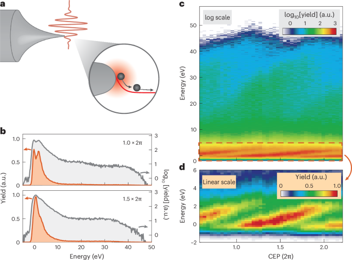
For the measurement shown in Fig. 1, we used a step size of 0.26 rad in CEP and recorded 105 electrons per phase step over a range of ~1.6 × 2π at a near-field peak intensity of 2.1 × 10¹³ W cm−2. We determine this intensity from the measured cut-off position of 42 eV.
Depending on the exact count rate and the CEP range, we can record a full map like that in Fig. 1 on the few-minute timescale. We note, however, that the electron emission yield and the spectra are typically very stable on the hour timescale. Here we profit from the low repetition rate of our laser system compared with typical oscillators operating around 80 MHz, which leads to fewer heating effects and consequently longer lifetimes of the metal needle tips.
We match the CEP axes (offset) of the experiment and theory based on a two-dimensional convolution of the low-energy region, exactly where the NILES feature shows up, similar to schemes that use the cut-off position or the photoionization yield13,54,55,56,57,58. The resulting phase error of this scheme can be as low as 120 mrad.
Analytical form of the MEC
We consider the ponderomotive energy at the tip surface (that is, in the maximally enhanced field and defined for peak field strength) as
$${U}_{{\rm{P}}}={\xi }_{0}^{2}{U}_{{\rm{P}}}^{\;{\rm{inc}}}={\xi }_{0}^{2}\frac{{e}^{2}{E}_{0}^{2}}{4m{\omega }^{2}}={\xi }_{0}^{2}\frac{{e}^{2}{I}_{0}}{2c{\epsilon }_{0}m{\omega }^{2}},$$
where \({U}_{{\rm{P}}}^{{\rm{inc}}}\) is the ponderomotive energy of the incident laser pulse without field enhancement.
Considering the temporal intensity envelope and the spatial near-field profile, the dynamical (spatiotemporal) ponderomotive energy reads
$${U}_{{\rm{P}}}(x,t)=\xi {(x)}^{2}\frac{{e}^{2}I(t)}{2c{\epsilon }_{0}m{\omega }^{2}}.$$
This results in the (also spatiotemporal) ponderomotive force
$${F}_{{\rm{P}}}(x,t)=-\frac{\,\text{d}}{\text{d}\,x}{U}_{{\rm{P}}}(x,t)=-\frac{{e}^{2}I(t)}{2c{\epsilon }_{0}m{\omega }^{2}}\times 2\xi (x){\xi }^{{\prime} }(x).$$
Solving this equation yields the drift trajectories shown in Fig. 2, which include the full near-field decay but neglect the oscillations of the optical field because we average over one optical cycle. Note that electrons start one quiver length away from the surface in the drift picture.
As an upper estimate, we now only evaluate the ponderomotive force at the surface, where ξ(x = 0) = ξ0 and \({\xi }^{{\prime} }(x=0)={\xi }_{0}^{{\prime} }\), and find the temporal ponderomotive force at the surface as
$${F}_{{\rm{P}}}^{\;{\rm{surf}}}(t)=-\frac{{e}^{2}I(t)}{2c{\epsilon }_{0}m{\omega }^{2}}\times 2{\xi }_{0}{\xi }_{0}^{{\prime} }.$$
The final momentum of an electron starting at rest at birth time tb follows from the integration of the classical equation of motion and yields
$${p}_{{\rm{final}}}({t}_{\mathrm{b}})=-2{U}_{{\rm{P}}}^{\;{\rm{inc}}}{\xi }_{0}{\xi }_{0}^{{\prime} }{\mathcal{F}}({t}_{\mathrm{b}}),$$
where \({\mathcal{F}}({t}_{\mathrm{b}})=\frac{1}{{I}_{0}}\mathop{\int}\nolimits_{{t}_{b}}^{\infty }I(t){\rm{d}}t\) is the remaining normalized pulse fluence the electron may experience after its birth into the optical field.
The drift energy of the electrons then reads
$${E}_{{\rm{final}}}({t}_{\mathrm{b}})=\frac{2}{m}{\left({U}_{{\rm{P}}}^{\;{\rm{inc}}}{\xi }_{0}{\xi }_{0}^{{\prime} }\right)}^{2}{{\mathcal{F}}}^{2}({t}_{\mathrm{b}}).$$
Trajectory simulations
One common way to simulate the electron energies of electrons triggered from metal needle tips is based on the three-step model4,5,43. It is based on a three-dimensional semiclassical point-particle trajectory analysis and allows us to simulate the electron energies for different laser intensities, as a function of CEP, and for spatially inhomogeneous optical fields. The initial conditions of the electrons in the three spatial dimensions are given by the projection of a two-dimensional Gaussian distribution on a hemisphere to model the tip. The starting times and the yield of the electrons are based on a closed-form quantum-mechanical model, often called the Yudin–Ivanov rate50,59. Originally, this model was developed for the electron emission from atoms. The metal–vacuum interface at the tips breaks the symmetry as compared with an atom. We assume, therefore, that electron emission takes place only in negative half-cycles as we are in the subcycle tunnelling regime (Fig. 4d). To avoid Coulomb repulsion effects, we artificially set the total rate to one electron per pulse in these simulations. After the emission, the electrons are propagated classically by numerically integrating the equations of motion based on a standard fourth-order Runge–Kutta scheme. Here we take into account the static field applied to the tip as well as the oscillating field. We model the static field using a spherical capacitor with the outer sphere set to infinity60. We choose Utip = –10 V as the bias voltage for all our simulations, if not specified otherwise. This voltage leads to a static field of 1 V nm−1 at the apex of the tip. For the oscillating near field, we choose a pulse with a Gaussian envelope representing the laser pulse given by
$$\begin{array}{rcl}E(r,t)&=&\exp \left(-\frac{2\ln (2){t}^{2}}{{\tau }^{2}}\right)\cos \left(\omega t+{\varPhi }_{{\rm{CEP}}}\right)\\ &&\times \left[1+({\xi }_{0}-1)\exp \left(-\frac{r}{\zeta }\right)\right].\end{array}$$
Here the pulse duration τ is given as the intensity FWHM. We chose a near-field shape with a decay constant of ζ = 10 nm, unless stated otherwise. For the simulations shown in Fig. 3a–c, the field enhancement factors chosen for the simulation are ξ0 = 1 (Fig. 3a), ξ0 = 7 (Fig. 3b) and ξ0 = 15 (Fig. 3c). We chose these values to account for the fact that the field enhancement factor increases for decreasing tip radius.
Extended Data Fig. 3a shows the CEP-resolved energy spectrum as obtained from the simulation. We colour code the emission distributions from the different optical cycles, where each colour corresponds to a specific cycle and the rate is given by the opacity of each colour. Extended Data Fig. 3b–d depicts which optical cycle corresponds to which colour for three different CEP values. This illustration clarifies that the number of NILES corresponds to the number of emitting cycles. Furthermore, we find that the lowest-energy part from –1 to 1 eV is dominated by the purple emission burst for a CEP of ~1.7 × 2π to 2.3 × 2π, for example. This is the basis to obtain a single attosecond emission burst (Fig. 4).
Parameter dependencies of the MEC
Figure 2e shows how NILES arises for one set of parameters, when the near field is inhomogeneous. Here the MEC (solid lines), representing the origin of NILES, is influenced by all parameters that change the optical field the electron experiences as it performs a quiver motion.
Extended Data Fig. 4a–c shows the dependence of the MEC on the most relevant parameters: peak optical near-field intensity, near-field decay length ζ and laser pulse duration τ. We discuss these parameters in the following. We use ζ = 10 nm, τ = 11.5 fs, a near-field intensity of 2.3 × 10¹³ W cm−2, a central wavelength of 1,570 nm and a tip voltage of –10 V, if not stated otherwise.
To quantify the effect of these parameters on NILES, we further calculate the maximum amplitude for each MEC, given by the difference in the maximum energy and minimum energy. We refer to this amplitude as the MEC amplitude and show these amplitudes in Extended Data Fig. 4d–f.
We find that the MEC amplitude increases for increasing intensity (Extended Data Fig. 4a). Extended Data Fig. 4a shows that it does so in a linear fashion. This increase reflects that the electrons are driven further away from the surface in the optical near field with increasing intensity; thus, they experience a larger variation in the optical near field, leading to an enhanced NILES effect. We note that this linear scaling is similar to the scaling of the low-energy peak for one fixed emission time, investigated in ref. 28. We further note that for our set of parameters, NILES is not detectable in the multiphoton region, as the amplitude would be too small to be detected for γ > 2.
When we sweep ζ from 150 nm (dark blue) towards smaller decay lengths (Extended Data Fig. 4b), we first observe an increase in the MEC amplitude, down to a value of ζ = 13.3 nm (green curve). When ζ is further decreased, however, the amplitude reduces again. Physically, this reduction is a consequence of an increasingly strong quenching of the quiver motion for smaller decay lengths, that is, the amplitude of the oscillatory motion decreases.
Extended Data Fig. 4c shows the MEC for different pulse durations τ. Although the amplitude of the MEC only slightly increases with a decreasing pulse duration (Extended Data Fig. 4f), the width of the MEC clearly broadens for longer pulses. This broadening along the time axis is to be expected, as the MEC is mainly affected by the time that the electron needs to escape the optical near field, as well as the optical pulse duration. In the limit of an infinitely long pulse, that is, the continuous-wave case, the MEC would be constant above zero for our case, because without the temporal envelope, all electrons born with a time difference of one optical period traverse the same near field. In the other case of constant pulse duration and increasing ζ, the NILES amplitude vanishes to zero (Extended Data Fig. 4b).
Influence of static electric fields
NILES is an effect entirely based on the quickly decaying optical near field. However, the shape and amplitude of NILES are influenced by the static bias field at the tip apex occurring when biasing the tip with a voltage Utip. This voltage results in an additional contribution to the final electron energies of Ed.c. = e × Utip, which we subtract when displaying the energies in our plots. To show this influence in more detail, we simulate the final energies of electron trajectories for four different cases: with and without a static field for a homogeneous field (ζ = ∞, ξ0 = 1) and a decaying near field (ζ = 10 nm, ξ0 = 10). The low-energy part of these simulations (Extended Data Fig. 7) reveals that only in the presence of a static field, energies below zero (that is, the final kinetic energies below Ed.c.) can be reached.
This result may be surprising when one thinks about an electron emitted without a laser field that surfs down only the static potential, leading to an energy of Ed.c. (in our case, 10 eV). It is the interplay of the laser-induced near field and the static field that enables emission with final energies below the d.c. voltage. However, this effect can only be observed clearly in the case of a strong inhomogeneity of the static field, given by the small dimensions of the tip.
Analogous to the MEC shown in Fig. 2e, the result including a static potential like in the experiment is shown in Extended Data Fig. 9, illustrating its effect on the NILES shape.
Extraction of momentum width
For the extraction of momentum width, we simulated the spectra similar to that detailed above with minor modifications to the model. First, we weighted the trajectories using the Wentzel–Kramers–Brillouin tunnelling rate. Second, we include the experimental energy resolution of the detector in the simulations. The resulting low-energy spectral features (Extended Data Fig. 5a) qualitatively capture the experimental NILES signatures (Extended Data Fig. 5c), but do not agree quantitatively. For a quantitative reconstruction, we further modify our simulations and perform an optimization (Nelder–Mead simplex method) for three additional parameters: first, the width σp of a Gaussian momentum distribution that we associate with each trajectory after propagation; second, the exponent n of a now considered exponential ionization rate R = En(x = 0, t), where E(x = 0, t) is the locally enhanced electric field at the surface; and third, a random CEP shift φCE. In this way, we optimized for the best overlap between the simulated and measured low-energy region of the spectra, including the NILES features. Out of 100 initial conditions for the optimization the best agreement (compare Extended Data Fig. 5b,c) was found for σp = 4.8 × 10⁻²⁶ kg m s−1 = 0.024 a.u., n = 4.24 and φCE = 0.05π. Especially including the momentum width paves the way to examine inter- and intracycle interference effects to a large extent with extended semiclassical simulations43.
CEP-dependent current
A CEP-dependent current is of the highest interest for direct CEP locking of lasers without the need of nonlinear interferometers. Although CEP-dependent currents have been demonstrated, so far they are too small for direct CEP locking13,22,30,32. In the following, we illustrate how NILES can be used to realize such a device, based on the direct electrons and, thus, with a much larger fraction of electrons contributing to the CEP-dependent current.
Extended Data Fig. 6a shows again the results of the measurement similar to Fig. 1b, from which we select two energy bands for the rescattered (blue) and direct (red) electrons. The chosen energy band for the rescattered electrons is 40–60 eV and 0.4–1.2 eV for the direct electrons. Extended Data Fig. 6b,c shows the integrated yield of the electrons of these bands, which both show a sine modulation as a function of the CEP. Although the modulation depth for the direct electrons is 33% and, thus, smaller than 46% for the rescattered electrons, the total yield of the direct electrons is 17 times higher than rescattered electrons. Hence, in total, NILES yields an approximately nine times better signal-to-noise ratio (SNR) than the rescattered electrons.
To stabilize a laser oscillator, an SNR of 30 dB at a bandwidth of 100 kHz is required61,62. Assuming this bandwidth and a repetition of 80 MHz, we obtain an SNR of 8 dB for NILES, too low for stabilization by a factor of over 100 in current. However, using a nanotip array, the current can be directly enhanced by orders of magnitude63. We foresee that this scheme can even be miniaturized to fit into the package of a small standard photodiode. There are already systems that measure the CEP based on the electron emission in a planar tip or bow-tie antenna configurations32,64,65. Especially for more than two-cycle laser pulses the integrated CEP-modulated current of such devices is small, leading to a small SNR. By using NILES and energy filtering, the sensitivity of such schemes can be considerably improved. Choosing an even larger energy window for the low-energy electrons (Extended Data Fig. 6), for example, the CEP-modulated current decreases, which is exactly what happens when measuring the integrated CEP current. Further, it was shown that for certain peak intensities, the CEP sensitivity of the integrated current can drop by over an order of magnitude, the so-called vanishing points32. This drop results from equally strongly emitting cycles within the laser pulse for different CEPs. Because of the energy shift of the different cycles, NILES can energetically separate different cycles and help to avoid such CEP-insensitive points.
Effect of near field on rescattered electrons
Figure 3 shows the influence of different optical near fields on NILES. Extended Data Fig. 8 shows the same simulations but on a logarithmic scale and a larger energy range, including the plateau electrons.
For the homogeneous case (Extended Data Fig. 8a), the direct electrons in the low-energy range do not show any CEP dependence, as expected. Yet, the tell-tale feature of strong field physics, the plateau, is shown, like the two others (Extended Data Fig. 8b,c). Since the actual waveform determines the maximum achievable energies, we observe a modulation of the highest energies as a function of the CEP, leading to the well-known arches in the cut-off region54. The electron energy spectrum in the homogeneous case reaches up to the expected ten times the ponderomotive energy UP of the laser field, that is, roughly 42 eV (ref. 6).
This cut-off energy cannot be reached for the inhomogeneous near-field profiles (Extended Data Fig. 8b,c), because of a quenched quiver motion19. This energy reduction is even better visualized by observing the final energies from one optical cycle (Extended Data Fig. 9a), where the maximum energies only reach 8.3UP for the chosen parameters. In addition, the reduced near field leads to a delayed starting time of rescattering (Extended Data Fig. 9a, stars).
The energy reduction demonstrates by how much NILES is different: although the optical near field affects only the energy of the rescattered electron, its presence changes the spectral structure of direct electrons completely.
Further, the simulations depicted in Extended Data Fig. 8a–c show that the near-field decay changes the CEP \({\phi }_{\max }\) at which the electrons are born that reach the highest energies (indicated by coloured arrows).
To determine \({\phi }_{\max }\) experimentally, we recorded further spectra with a CEP step size of 0.26 rad over a range of more than three periods with 5 × 10⁵ electrons per phase step and rate of 0.4 electrons per pulse (Extended Data Fig. 10a). We determine the cut-off position for each CEP by fitting two linear functions to the plateau and cut-off region13,38.
We fit a sine to the determined cut-offs (Extended Data Fig. 10a) and find an experimental value of \({\phi }_{\max ,\exp }=1.8\pm 0.5\) rad and a cut-off position of 40.7 eV with a modulation depth of 5.4 ± 0.2 eV (twice the amplitude of the sine fit). The resulting near-field intensity in this measurement is then 2.0 × 10¹³ W cm−2.
Extended Data Fig. 10b shows the simulated phase \({\phi }_{\max }\) as a function of ζ. We find that \({\phi }_{\max }\) monotonically decreases for increasing ζ. We observe that \({\phi }_{\max }(\zeta )\) is matched by a power law, where the offset is given by the homogeneous field case, with a phase of ϕmax(ζ→∞) = 0.9 rad. The measured phase of 1.8 ± 0.5 rad matches the simulated data within the error bars (black dot).
Because the experimentally determined phase \({\phi }_{\max ,\exp }\) is 0.9 rad larger than the simulated case with a homogeneous optical field (ζ = ∞), we see that the CEP at which the highest electron energies are created cannot be considered constant in the presence of an optical near field. This result shows that schemes measuring the CEP by the cut-off electrons clearly have to take decaying near fields into account. If not, the CEP can be grossly misinterpreted.
Moreover, the evaluated modulation depth of the cut-off of 5.4 ± 0.2 eV serves as an intrinsic measure for the near-field pulse duration present at the tip’s apex. The modulation depth is in good approximation given by the difference in the ponderomotive energies associated with the maximum field at CEP = 0 and CEP = π, for one fixed pulse envelope. Extended Data Fig. 10c shows the modulation depth as a function of the cut-off energy, that is, ten times the ponderomotive energy, and the pulse duration. On the basis of this map, the experimental pulse duration is 11.1 ± 0.4 fs, in good agreement with the FROG-based measurement of 11.5 fs.
Similar maps can be generated using the semiclassical simulation including both optical near field and static field. The map produced by such a simulation gives a pulse duration of 11.5 ± 0.4 fs, perfectly matching the result from FROG. The better agreement is due to the fact that quenching effects are not taken into account when we only consider the difference in ponderomotive energies at CEP = 0 and CEP = π. However, we emphasize that using this difference provides experimenters with a simple tool to measure the pulse duration within the typically required accuracy in the experiment, without the need for simulations.
Impact of coherent phenomena on NILES
So far, all simulations were based on a semiclassical treatment in which only the emission process was modelled quantum mechanically. To rigorously include quantum interference and quantum diffusion, we now simulate the energy spectra based on a numerical solution of the one-dimension time-dependent Schrödinger equation (TDSE)15,39. We obtain the wavefunction of the electron by integrating the TDSE numerically by a Crank–Nicolson method (details and code are provided in ref. 15). As the ground state, we assume an electron that is bound in a box potential with a half-sided linear decaying potential, mimicking the static potential present at the tip. The potential is chosen such that the electron has an energy of 20 eV without any laser field after traversing the full potential. The width of the box is chosen to match the work function of tungsten, which we assume as 6 eV (ref. 15). The assumption of a single bound state may seem surprising because metals have, in general, many available states that are occupied according to the Fermi–Dirac distribution. However, because of the high nonlinearity of the electron emission, one energy level will be dominant and all other lower-lying states are strongly suppressed66.
Extended Data Fig. 10d shows the result for an incident intensity of 1.8 ×10¹³ W cm−2, ζ = 10 nm and ξ0 = 5, similar to the experiment shown in Extended Data Fig. 10a. The main features of the simulated spectrum are very close to the spectra simulated with the semiclassical model. However, the TDSE is fully coherent; hence, we find multiphoton photoemission (MPP) peaks spaced by the photon energy, effectively visible as fine stripes over the entire spectrum. NILES also shows up in the low-energy region, smoothly transitioning into the spacing of the MPP peaks above 2 eV (Extended Data Fig. 10e). It is interesting to note that the whole low-energy region (–1 to 5 eV) experiences a CEP-dependent energy shift similar to the shape of NILES, even above 2 eV in which we classically observe no NILES feature. The fact that the semiclassical and quantum simulation agree except for the appearance of MPP peaks shows that the dynamics of the emitted electron wave packets is dominated by the centre-of-mass motion in the optical near field (Ehrenfest dynamics).
In the experiment, we have so far not observed MPP peaks together with NILES, which can be for two reasons. For longer pulse durations without CEP variation, we have measured such MPP peaks already in the same setup67. The broader bandwidth of our few-cycle laser pulses in the present case broadens the width of MPP peaks68. Further, the coherence time at such high intensities is possibly reduced so heavily that already two emission events in two consecutive cycles cannot interfere anymore. Investigating details of the electron coherence will be the subject of future work.