Passive air sampling detects environmental DNA transfer from water into air

Field sampling

We conducted this study near Seattle, Washington USA, in Issaquah Creek, a salmon spawning stream, outside of the Issaquah Salmon Hatchery (47.529501°N, 122.039133°W) from 17 October 2024 to 21 November 2024, with six sampling events. Issaquah Creek is a tributary of Lake Sammamish that drains approximately 175 km2 of mixed forested and urban watershed in the Cascade foothills, with discharge of 30–50 cfs (0.8–1.4 m \(3\)/s) during the study period. The creek supports natural runs of Chinook and Coho salmon, with the Issaquah Salmon Hatchery operating at this location since 1936. The study site was in a riparian corridor approximately 3 km upstream from the creek’s mouth at Lake Sammamish, where the watershed transitions from forested headwaters to developed lowland areas.

We sampled at six time points that spanned the entire Coho salmon (Oncorhynchus kisutch) run, from the first arrivals in early fall of August through peak abundance around 17 October 2024 and into the tail end of the migration in November. This schedule ensured that our eDNA sampling captured both the lowest and highest levels of fish activity. Within the same sampling period, visual fish counts were performed by the hatchery staff, and salmon escapement data were obtained from the Washington Department of Fish and Wildlife escapement reports (https://wdfw.wa.gov/fishing/management/hatcheries/escapement#2024-weekly). The hatchery operates a fish ladder with gates that are opened periodically by staff, who conduct visual counts of accumulated fish before allowing passage. This controlled system ensures that all Coho salmon in the study area are counted at this single point before entering the hatchery, creating a direct correspondence between visual counts and the fish population generating eDNA signals in our sampling area. Weather conditions varied throughout the sampling period; environmental metadata for each sampling date – precipitation and mean daily river discharge – are provided in (Table. S2).

Airborne eDNA sampling

Sampling for eDNA was conducted in 24-h blocks with deployment and recovery around 9 a.m. (river water was collected only on the first day of each of the six sampling timepoints). Four passive collection methods were evaluated: three filter types – gelatin (Sartorius, 47 mm diameter), PTFE (Whatman, 47 mm diameter), and MCE (Sterlitech, 5.0 \(\mu\)m pore size, 47 mm diameter) – and an open container of deionized water. The rationale for selecting these materials was as follows: gelatin filters are effective at capturing airborne particles and are particularly suited for applications where maintaining viability (e.g., for subsequent bacterial culturing35😉 is desired; PTFE filters are noted for their high durability and are widely used in active air sampling experiments36; whereas MCE filters, typically employed for water filtration, were included to assess their performance in an airborne context7. All three passive filters were deployed via custom 3D-printed “honeycomb” puck filter holders, based on open-source Thingverse designs (IDs 4,306,478 and 979,318; Zachary Gold, pers. comms.), and were suspended from a hatchery railing approximately 3 m above the river water level (Fig. 1), with their collection surfaces oriented vertically. This configuration minimized splash contamination and captures airborne DNA particles driven by gravitational settling. The positioning relative to flowing water demonstrated how these passive collectors operate at a vantage point above the stream, facilitating non-invasive DNA capture in real-world field conditions. Two biological replicates were deployed for both gelatin and PTFE, while only one replicate was used for MCE. After the overnight deployment, filters were carefully recovered using sterile, disposable forceps and immediately immersed in 1.5 mL of DNA/RNA Shield.

Fig. 1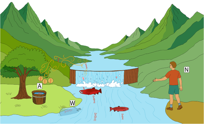

Conceptual illustration of cross‐medium eDNA sampling above a salmon‐spawning stream. Natural processes, including evaporation, bubble-burst aerosolization at riffles and splashes, and the vigorous movement of spawning Coho salmon, launch trace amounts of DNA from the river surface into the atmosphere. Passive airborne samplers, shown here as three vertically hung filters and an open tray of deionized water (A), intercept settling airborne eDNA, while paired water-grab sampling (W) and visual counts by hatchery staff (N) provide concurrent reference measurements.

The fourth passive collection method was an open container (25 cm width, 30 cm length, 10 cm depth) filled with 2 L of deionized water18 also positioned about 3 m above the river and about 30 cm above the suspended passive filters. The open container was also deployed for about 24 h at the same times as the passive filters. The container had an open surface (i.e., oriented horizontally) to capture airborne particles settling by gravity. The surface area of the container was approximately 750 cm2, in contrast to the roughly 16 cm2 surface area offered by the 47-mm circular filter disks. Only one replicate was used for the open water container method. Note that although 2 L of deionized water was placed in the container, heavy rainfall during overnight deployments sometimes increased the water level. Any debris (e.g., bugs, leaves) was removed from the container before on-site filtration using the same system as for river water samples (see below for details).

Water eDNA sampling

At each of six sampling events, we collected one 3 L surface-water grab (3 × 1 L biological replicates) at a fixed site immediately downstream of the fish-ladder gate, adjacent to the Coho salmon aggregation area and concurrent with air deployments. Water was collected in sterile bottles, directly adjacent to the aggregation area. The ladder is operated continuously by hatchery staff throughout the salmon run, ensuring fish passage and visual counts. A total of 3 L of water was filtered on site using a Smith-Root Citizen Science Sampler equipped with 5.0 \(\mu\) m mixed cellulose ester (MCE) filters7. Three 1 L replicates were processed and immediately preserved in 1.5 mL of DNA/RNA Shield (Zymo Research) using clean disposable plastic forceps. Field-negative filtration blanks (1 L of Milli-Q water each) were also processed using the same system. All equipment was decontaminated with 10% bleach, thoroughly rinsed with deionized water, and handled with gloves to minimize contamination. All filters (passive air, passive open container, water) were stored at –20°C until processing, typically within one week.

The ladder site concentrates upstream migrating Coho salmon and is the control volume where fish are enumerated; sampling water at this location keeps measurements co-located with the airborne collectors and the visual count. One 3 L sample per event provided six time-matched water–air pairs for estimating the water-to-air transfer parameter \(\eta\) in the joint model (see Sect. 2.5). In this design, water serves as a calibrated comparator for airborne eDNA34,37. This single water sample per event was the paired water measurement used in the joint model.

Wet-Laboratory procedures

DNA extraction from both river water samples and airborne filter samples was performed using the Qiagen Blood and Tissue Kit according to the manufacturer’s protocols. During extraction, it was noted that the gelatin filters dissolved completely in the DNA/RNA Shield. Samples were vortexed for 1 min, and 500 \(\mu\) L of the shield was used for DNA extraction.

qPCR assays targeted a 114-bp fragment of the cytochrome b gene of Coho salmon, using the forward and reverse primers derived from Duda et al.38 – COCytb_980-1093 Forward: CCTTGGTGGCGGATATACTTATCTTA and COCytb_980-1093 Reverse: GAACTAGGAAGATGGCGAAGTAGATC. Although Duda et al. validated a TaqMan (probe-based) assay, we used SYBR Green chemistry with the SYBR Select Master Mix (Fisher Scientific) and verified specificity by melt-curve analysis; on an Applied Biosystems QuantStudio 5 real-time PCR system with a 384-well block. Each 10 \(\mu\) L reaction consisted of 5 \(\mu\) L of SYBR Select Master Mix, 0.4 \(\mu\) L of 10 mM forward primer, 0.4 \(\mu\) L of 10 mM reverse primer, 2.2 \(\mu\) L of molecular grade water, and 2 \(\mu\) L of DNA template. Melt curve analysis was performed to confirm the amplification of the target fragment, with an accepted melting temperature of 81 °C ± 1°C. All standards and positives showed a single melt peak at 81 °C ± 1 °C, and no-template and field-negative controls showed no amplification.

Standard curves were constructed using a Coho salmon tissue DNA extract quantified with a Qubit fluorometer (Figure S6). The stock solution was diluted to 1.0 ng/\(\mu\) L and designated as 106 copies/\(\mu\) L. Serial dilutions were then prepared, with 105, 104 and 103 copies/\(\mu\) L run in triplicate, 102 copies/\(\mu\) L in quadruplicate, and 101/\(\mu\) L copies in triplicate. Assay performance was summarized by the qPCR standard curve and a detection-probability curve derived from replicate standards (Figure S6), and this observation-level uncertainty was propagated in the hierarchical model; accordingly, we reported these performance curves rather than fixed LOD/LOQ thresholds.

Joint statistical modelVisual observation model

In summary, we synthesized three methods of observations (visual counting of fish, water eDNA measurements, and air eDNA measurements) that derived from a single unknown true fish accumulation rate (denoted here as \(X\)). This joint approach allowed us to estimate the aerosolization factor (\(\eta\); the fraction of water eDNA transferred to air), the effectiveness and reliability of different passive air filtering techniques (\(\tau\)), and the replicability of various filters (\(\rho\)) throughout the 6-week peak coho salmon spawning period. Accordingly, the water measurement at the fish ladder counting site was used as a time-matched index of local fish density that drove the air compartment in the joint model. At each sampling event, we obtained one water measurement at the ladder site and contemporaneous air measurements from the passive air collectors (by filter type with biological replicates). The aerosolization parameters were estimated from the six paired water–air observations across the study period.

We modeled the upstream migration of Coho salmon (Oncorhynchus kisutch) as arising from the inferred unknown true density of fish, X. As individuals moved upriver, fish accumulated in a holding area immediately downstream of the hatchery river dam (our water and air sampling location). At discrete times \(t\) (six weekly sampling dates between 17 October and 21 November 2024), the hatchery staff opened the ladder gate to allow passage into holding tanks. Between successive gate-opening events (\(\Delta t\)), additional coho salmon arrive and join the backlog in the holding area, increasing the number of individuals awaiting passage. We denoted the true daily accumulation rate \({X}_{t}\) (also fish density at the river dam) in units of fish/day at time \(t\), and we denoted the counting effort as \(E\) (measured as the elapsed number of days between consecutive gate openings; \({E}_{t}=\Delta t\); hence \({E}_{t=1}=0\)). Here, \({E}_{t}\) (days) represented the count effort, converting the daily accumulation rate \({X}_{t}\) (fish/day) into the expected accumulated count \({\lambda }_{t}={X}_{t}\cdot {E}_{t}\) (fish) in Eq. (1). Counts were full enumerations at the ladder immediately before each opening and hence, person-hours are not modeled separately. Prior to each gate opening (at time \(t\)), the hatchery staff conducted a visual count \({N}_{t}\) of accumulated fish. Assuming \({X}_{t}\) remained relatively constant between successive gate-opening events (\(\Delta t\)), we modeled the observed fish counts as a Negative Binomial process:

$${\lambda }_{t}={X}_{t}\cdot {E}_{t}$$

(1)

$${N}_{t}\sim \text{Negative}\hspace{0.25em}\text{Binomial}({\lambda }_{t},\phi )$$

(2)

where, \(N\) was the visually observed number of fish at time \(t\), \({\lambda }_{t}\) was the expected number of fish accumulated over the \({E}_{t}\)-day interval with a fixed overdispersion parameter shared across time points (\(\phi =20\); hence variance \(\lambda +\frac{\lambda^2}{\phi }\))3,39. Given the small number of time points (n = 6), the overdispersion parameter \(\phi\) was fixed to a literature-supported value rather than estimated.

Molecular process model

We denoted \(W\) as the unobserved eDNA concentration (copies/L) in the single water sample collected at each time point \(t\) and \(\omega\) as the “integrated eDNA factor” – the conversion factor between fish accumulation (\(X\)) and eDNA concentration (\(W\); see Guri et al.3 for further interpretation of \(\omega\)). Here, \(\omega\) was treated as a population-scale factor that aggregated per-fish eDNA emission (i.e., the average shedding rate per individual), together with decay, transport, and dilution at the site; we assumed it was approximately constant over the 24-h sampling window. Individual-to-individual variation was not modeled explicitly and contributed to residual variance. We express the relation between the fish density and water eDNA concentration as:

$${W}_{t}={X}_{t}\cdot \omega$$

(3)

We denoted \(A\) as the unobserved eDNA concentration (copies/cm2/day) in the air at time \(t\) which was filtered using passive collection method \(j\). We indexed air collection methods as \(j\in \{1,\dots ,4\}\) index air-collection methods: 1 = PTFE, 2 = gelatin, 3 = MCE (air-suspended), 4 = DI-water tray. We modeled the air eDNA concentration as a log-linear function of the water eDNA with intercept \(\eta\), slope = 1, and error term \(\varepsilon\) (unexplained variability; time and filter specific):

$$\text{ln}({A}_{tj})={\eta }_{j}+\text{ln}({W}_{t})+{\varepsilon }_{tj}$$

(4)

Here, the intercept \(\eta\) was be interpreted as the water-to-air transferability (or dilution) factor and \(\varepsilon\) as the error term parameter (similar to the sum of squares error) from a linear regression where \({\varepsilon }_{tj}\sim \mathcal{N}(0,{\tau }_{j})\).

For the two filter types with biological replicates (\(j\in \{1,2\}\); PTFE and gelatin); we sampled two biological replicates and we used the mean of those biological replicates to determine the average concentration in the air \(A\) at time \(t\) as following:

$${ln}({A}_{tjb})=\text{ln}({A}_{tj})+{\delta }_{tjb} \quad {\text{for}}\hspace{0.25em}j\in \{1,2\}$$

(5)

where \({\delta }_{b}\) indicated the deviation of individual biological replicate from the average concentration (\({A}_{tj}\)), following a normal distribution with mean 0, \({\delta }_{tjb}\sim \mathcal{N}(0,{\rho }_{j})\), with \({\rho }_{j}\) indicating the magnitude of the replicates’ deviation from the mean sample. Because we had only two replicates at each sampled time, we imposed a sum to zero constraint on the replicates (\(b\)) collected from a single sampling time (\(\sum_{b}{\delta }_{tj}=0\)).

To estimate the levels of eDNA concentration in water (\(W\)) and air (\(A\)), we utilized the qPCR observation models (as described in Guri et al.37 and Shelton et al.34, with slight modifications). The model compartment utilized the standard curve samples to estimate the intercept (\(\phi ,\beta_0,\gamma_0\)) and slope (\(\beta_1,\gamma_1\)) parameters between the known concentration (\(K\)) and the observed data (\(Z\) and \(Y\)) from qPCR machine as follows:

$$Z_{kr} \sim \text{Bernoulli}(\psi_{k})$$

(6)

$$psi_{k} = 1 – \exp(-K_{k} \cdot \theta)$$

(7)

$$Y_{kr} \sim \text{Normal}(\mu_{k}, \sigma_{k}) \quad \text{if } Z_{kr} = 1$$

(8)

$$\mu_{k} = \beta_{0} + \beta_{1p} \cdot \ln(K_{k})$$

(9)

$$\sigma_{k} = \exp(\gamma_{0} + \gamma_{1} \cdot \ln(K_{k}))$$

(10)

where we denoted \(Z\) is the binary outcome of target amplification for sample (\(k\)) and technical replicate (\(r\)) being present (1) or absent (0) following a Bernoulli distribution given the probability of detection \(\psi\) for each sample (\(k\)). We denoted the parameter \(\phi\) as the intercept of the function between probability of detection \(\psi\) and the known DNA concentration (\(K\); copies/\(\mu\) L reaction) as the predictor variable. Additionally, for Eqs. 8–10, \(Y\) was the observed cycle threshold (Ct) for sample (\(k\)) and technical replicate (\(r\)) which followed a normal distribution with mean \(\mu\) (mean Ct) and standard deviation \(\sigma\) for each sample (\(k\)). We modeled \(\mu\) as a linear function of known eDNA concentration (\(K\)) with intercept \(\beta_0\) and plate specific (\(p\)) slope \(\beta_1\) and the standard deviation \(\sigma\) of the observed Y as an exponential function of known eDNA concentration with intercept \(\gamma_0\) and slope \(\gamma_1\).

Subsequently, we build the same model compartment for estimating eDNA concentration in water and air by substituting \({U}_{t}\) and \({Q}_{tj}\) (and \({Q}_{tjb}\) for \(j\in \{1,2\}\)) respectively, with \({K}_{k}\) through Eqs. 6–10 (see Figure S1), where \(U\) and \(Q\) are concentration normalized per reaction volume (\(V\) = 10 \(\mu\) L for all reactions including water and air samples), water volume filtered in the field (\(F\) = 1 L for all water samples), surface area (\(S\) = 16 cm \({}^{2}\) for gelatin, PTFE, and MCE, and 750 cm2 for the open containers of deionized water; for air samples only), and for passive deployment time (\(P\) = 1 day across all samples at all time \(t\); for air samples only) of \(W\) and \(A\) respectively as follows:

$${U}_{t}={W}_{t}\cdot F/V$$

(11)

$${Q}_{tjb}={A}_{tjb}\cdot {S}_{tj}/V\cdot P$$

(12)

The intercept and slope parameters (from Eqs. 7, 9, and 10) between qPCR observations and eDNA concentration of water, air and the standard samples were shared between model compartments.

Model conditions

The joint model (Figure S1) was implemented using the Stan language as implemented in R (package: Rstan) running four independent MCMC chains using 5000 warm-up and 5000 sampling iterations (for parameters and their prior distributions see Table S1). The posterior predictions were diagnosed using statistics40 and considered convergence for values less than 1.05 and effective sample size (ESS) greater than 1000 for all parameters. Additionally, the posterior predictive checks were used with results presented in the Figure S5. Observations from different gate-opening intervals were assumed independent; with n = 6, we did not fit an explicit temporal correlation structure.