
In this section, we provide the proposal for machining process dynamics rooted in energy variation. Some key techniques are described, such as microstate decomposition and importance weighting. Besides, the overall framework and model structure of the proposed method for dynamics discovery are discussed in detail. Followed by the validation of the effectiveness of the proposed methodology by three machining cases.
Microstate definition
The machining signals are typical non-stationary signals, with the statistical characteristics varying over time. A complete time-varying state can be represented as a superposition of multiple micro components with instantaneous frequencies:
$${X}\left(t\right)={\mathrm{Re}}\left\{\mathop{\sum }\limits_{n=1}^{N}{A}_{n}\left(t\right){e}^{j{\int}_{0}^{t}{\omega }_{n}\left(\tau \right)d\tau }\right\}$$
(1)
In which, \({\mathrm{Re}}\{\cdot \}\) denotes the real part, \(n\) denotes the component index, \({A}_{n}\) and \({\omega }_{n}\) are the instantaneous amplitude and frequency of the \(n\)-th component, respectively, and \(j\) is the imaginary unit. Considering continuous time \(t\) as a discrete time instant \(i\), there is:
$${X}_{i}=\mathop{\sum }\limits_{n=1}^{N}{{\boldsymbol{C}}}_{n,i}$$
(2)
In which, \({{\boldsymbol{C}}}_{n,i}={\mathrm{Re}}\left\{{A}_{n,i}{e}^{j{\int}_{\!0}^{i}{\omega }_{n}d\tau }\right\}={\left\{{{\boldsymbol{c}}}_{i}\right\}\,}_{n=1}^{N}={\left\{{{\boldsymbol{c}}}_{n}\right\}\,}_{i=1}^{k}\) represents the \(n\)-th component at the \(i\) moment. Based on the definition above, the microstate vector \({{\boldsymbol{c}}}_{i}\) at any given moment is considered as a specific instance of sampling from the probability distribution at that current moment:
$${{\boldsymbol{c}}}_{i} \sim p\left(E\left({{\boldsymbol{c}}}_{i}\right)|{Z}_{i}\right)$$
(3)
In which, \({E}_{i}\) and \({Z}_{i}\) denotes the energy and partition function of the instantaneous microstate at the \(i\) moment, respectively. They collectively govern the probability density function of microstates \(p\) at the current instant.
Energy feature
The accurate establishment of the above energy feature in the cutting process is critical for further analysis. According to the general laws derived from statistical mechanics for a system33, the system’s total energy is considered as only the sum of the energies of numerous microstates. However, this perspective does not hold during the machining. Microstates are recognized to have varying contributions to the macrostate.
For instance, it has been experimentally demonstrated that apart from the milling force components strongly correlated to the state of tool wear, i.e., the domain frequency within 400–700 Hz and the harmonics of the tooth passing frequency, the original collected signals also contain multiple information including tool runout, the state of machine tool, and noises persist throughout the entire machining process but weakly correlated to the assessment of tool wear34. Similarly, the trend component and the emergence of new frequency components are more closely related to chatter, rather than the general periodic components35. This correlation can generally be obtained through statistical analysis, including correlation analysis36 and principal component analysis37, in addition to first principles.
Therefore, the different scales within one signal typically contain information that can reveal the machining conditions. As it has been demonstrated by Peng34 and Wang38 that multi-scale features could capture more inherent relationships in cutting processes than from a single-scale perspective. To this end, it’s not advisable to completely remove certain components, firstly as they may not be completely eliminated, and secondly as the removal may lack sufficient accuracy. In contrast, assigning weights to them is more reasonable, as it allows for retaining certain essential components while reducing the importance of certain irrelevant ones. The energy of microstates is represented as follows:
$${E}_{i}=\mathop{\sum }\limits_{n=1}^{N}{w}_{n,i}{{\boldsymbol{C}}}_{n,i}^{2}$$
(4)
In which, \({w}_{n}\) represents the importance of the \(n\)-th component of the microstate vector. This feature metric is represented by the squared amplitude of the signals.
Macrostate estimation
The microstates possess extremely short relaxation times with their distribution \(p\) can be computed under known statistical laws. It has been shown by Xu et.al.39 that the energy distribution of different components of the cutting signal exhibits an exponential trend, which suggests an underlying distribution mode analogous to the Boltzmann distribution. Therefore, the instantaneous statistical distribution can be approximated by the Boltzmann distribution:
$$p\left(E\right)=\frac{{e}^{-\beta E}}{Z}$$
(5)
In which, \(\beta\) is the Boltzmann constant.
The uncertainty of this distribution is measured by entropy and represented as:
$${S}_{i}=-{p}_{i}{{log}_{2}}\left({p}_{i}\right)$$
(6)
Subsequently, the machining dynamics can be reflected through variations in the underlying patterns of the data feature like energy, partition, and entropy. For instance, unsupervised learning uncovers that the tool condition can be identified from feature clustering20. The patterns within the data are strongly correlated with entropy40,41, thus allowing for the assessment of the macrostate of a machining system through the dimensionless measure of entropy:
$${a}_{i}=g\left({S}_{i}\right)$$
(7)
This framework aligns with our understanding of general manufacturing processes. From the perspectives of entropy and energy, numerous irreversible processes and abnormal phenomena, such as tool wear and chatter vibration, can be clearly explained. However, obtaining these characteristics necessitates the development of suitable mathematical models for the processes, which can be challenging to discover. Therefore, we have developed a mechanism-assisted method in the subsequent section.
Figure 1 presents the overall framework of the theory in this study. Theoretically, the cutting process’s sensor signals are modeled as a macrostate consisting of statistical averages of numerous series of microstates. At any given moment, the energy determined through microstate importance weighting defines the probability of specific microstate combinations, with its entropy and partition functions directly linked to the macrostate. By collecting sensor data and applying it to a specifically developed machine learning model, the changes in the microstate and the relationship among entropy, partition function, and machining state, thereby facilitating the monitoring of the machining state.
Fig. 1: The framework of the machining process dynamics.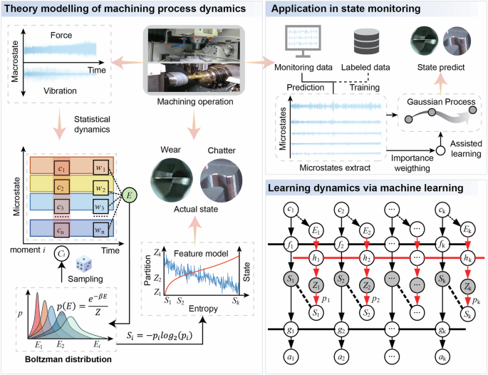
The left side illustrates the definition from microstates to macrostates, corresponding to the theoretical section; the right side demonstrates the application of the theory in processing, corresponding to the specific approach.
Dynamics discovery via mechanism-assisted Deep Gaussian Process
The dynamic process derived in theory is highly complex, complicating the identification of entropy and other dimensionless quantities. Machine learning provides an efficient solution approach to address this challenge.
The deep learning approach for discovering the dynamics employs Deep Gaussian Process as the baseline model, which is suitable for handling small datasets characterized by intricate mapping relationships and can deliver precise estimates of uncertainty. Unlike deterministic modeling approaches, probabilistic modeling can significantly enhance decision-making reliability by quantifying the inherent stochasticity in manufacturing processes42. A typical Gaussian Process could be represented as:
$$\left(\begin{array}{c}{\boldsymbol{y}}\\ {f}_{* }\end{array}\right){\mathscr{ \sim }}{\mathscr{N}}\left(\left[\begin{array}{c}{\boldsymbol{\mu }}\\ {\mu }_{* }\end{array}\right],\left[\begin{array}{cc}{\boldsymbol{K}} & {{\boldsymbol{K}}}_{* }^{T}\\ {{\boldsymbol{K}}}_{* } & {{\boldsymbol{K}}}_{* * }\end{array}\right]\right)$$
(8)
$${f|y},{\boldsymbol{X}},{{\boldsymbol{X}}}_{* }{\mathscr{ \sim }}{\mathscr{N}}\left({\mu }_{* }+{{\boldsymbol{K}}}_{* }{{\boldsymbol{K}}}^{-1}\left(y-\mu \right),{{\boldsymbol{K}}}_{* * }-{{\boldsymbol{K}}}_{* }{{\boldsymbol{K}}}^{-1}{{\boldsymbol{K}}}_{* }^{T}\right)$$
(9)
In which, \({\boldsymbol{X}}\), \({{\boldsymbol{X}}}_{* }\) represents observed target variables and new inputted variables, corresponds to the extracted signal features. \(y\) and \({f}_{* }\) represents the predicted outputs at training data and unseen inputs, corresponds to the continuous or discrete states of the machining process. \({\boldsymbol{\mu }}=\mu \left({\boldsymbol{X}}\right)\) represents the mean of GPR, \({\mu }_{* }=\mu \left({{\boldsymbol{X}}}_{* }\right)\), \({\boldsymbol{K}}=K\left({\boldsymbol{X}},{\boldsymbol{X}}\right)+{\sigma }_{n}^{2}{\boldsymbol{I}}\), \({K}_{* * }=K\left({{\boldsymbol{X}}}_{* },{{\boldsymbol{X}}}_{* }\right)\), \({K}_{* }=K\left({\boldsymbol{X}},{{\boldsymbol{X}}}_{* }\right)\), \({\sigma }_{n}^{2}\) represents the variance of signals and denotes the identity matrix.
Traditional deep learning models are purely data-driven approaches that establish uninterpretable black-box models linking inputs to final labels, which is disadvantageous for building models with clear process mechanisms and discovering their characteristic quantities. Therefore, we design an improved deep Gaussian process model applicable to discover the above dynamics in the machining process42. The model consists of two core modules: an importance-attribution block and a mechanism-assisted block.
Importance-attribution block
It is important to conduct decomposition first to get the machining process microstates. The results of traditional mode decomposition are purely data-driven. There is currently no unified theory or principle for selecting effective components from the Intrinsic Mode Functions (IMFs) derived from decomposition, nor for elucidating their relationship with macroscopic states. Generally, this selection process relies on subjective judgment, which is relatively complex to implement and overly dependent on human experience. This often leads to the inclusion of irrelevant components or high noise content, resulting in poor effectiveness in analyzing the state of the machining process. Therefore, a module is proposed that adaptively assigns importance based on the characteristics of the cutting signals. It utilizes mutual information (MI) entropy to assign weights, emphasizing the extraction of task-relevant microstates. Where the segment feature of each segment in process signals is stationary:
$$H\left({{\boldsymbol{c}}}_{{\boldsymbol{n}}},{{\boldsymbol{c}}}_{{{\boldsymbol{n}}}^{{\prime} }}\right)=p\left({{\boldsymbol{c}}}_{{\boldsymbol{n}}},{{\boldsymbol{c}}}_{{{\boldsymbol{n}}}^{{\prime} }}\right){\log }_{2}\left(\frac{p\left({{\boldsymbol{c}}}_{{\boldsymbol{n}}},{{\boldsymbol{c}}}_{{{\boldsymbol{n}}}^{{\prime} }}\right)}{p\left({{\boldsymbol{c}}}_{{\boldsymbol{n}}}\right)p\left({{\boldsymbol{c}}}_{{{\boldsymbol{n}}}^{{\prime} }}\right)}\right)$$
(10)
$${w}_{n}={\rm{Norm}}\left\{\mathop{\sum }\limits_{{n}^{{\prime} }=1}^{N}H\left({{\boldsymbol{c}}}_{n},{{\boldsymbol{c}}}_{{n}^{{\prime} }}\right)\right\}$$
(11)
In which, \(H\) is mutual information, \({\rm{Norm}}\left\{\cdot \right\}\) represents the normalization operation, \({w}_{n}\) denotes the weight of \(n\)-th IMF.
MI quantifies the nonlinear dependence between two microstates. Further, the total MI-based interdependence metric reflects the informational relevance of all microstates within a cutting system. The weights prioritize IMFs with strong interdependencies, as they exhibit strong MI with multiple others and may encode shared dynamical features, making them a salient contributor to the macrostate.
This module employed variational mode decomposition (VMD) to extract IMFs, followed by energy quantification through the above dedicated weighting module applied to each IMF. The optimization parameters and implementation specifics of the VMD algorithm are comprehensively described in the Method section.
The mechanism assistance
Machine learning is a robust tool that provides diverse methodologies for the exploration and analysis of the intricate structures and features within machining signals. Nevertheless, existing models exhibit a degree of rigidity in dealing with the specific issues, which limits our understanding of the actual dynamics. To address this limitation, a mechanism-assisted framework is proposed. This framework incorporates three Gaussian process layers designed to effectively capture the system dynamics: the state layer (which receives the microstate and outputs entropy), the mechanism-assisted layer (which receives the energy output partition), and the observation layer (which receives the entropy and outputs the system state).
In the state layer, the most widely used squared exponential kernel function is adopted, which can map original features into an infinite-dimensional space, thereby enhancing the likelihood of discovering complex patterns within the data. Among these, to better represent the distance between probability distributions, the Wasserstein distance is incorporated into the kernel function:
$$W\left({{\boldsymbol{c}}}_{i},{{\boldsymbol{c}}}_{{i}^{{\prime} }}\right)=\mathop{\inf }\limits_{\pi \sim \prod \left({{\boldsymbol{c}}}_{i},{{\boldsymbol{c}}}_{{i}^{{\prime} }}\right)}{{\mathbb{E}}}_{\left(u,v\right) \sim \pi }\left({||u}-{v||}\right)$$
(12)
$$k\left({{\boldsymbol{c}}}_{i},{{\boldsymbol{c}}}_{{i}^{{\prime} }}\right)={\sigma }^{2}\exp \left(-\frac{{W}^{2}\left({{\boldsymbol{c}}}_{i},{{\boldsymbol{c}}}_{{i}^{{\prime} }}\right)}{2{l}^{2}}\right)$$
(13)
Where, \(\pi\) denotes the joint probability distribution, \(u\) and \(v\) are sample points in the source space and target space, respectively. \(\sigma\) and \(l\) are model hyperparameters.
This strategy considers the spatial structure between distributions and the shapes of the two probability distributions, thereby enabling it to better capture their similarities.
Furthermore, we attempt to integrate physical modules into the machine learning framework. This innovative endeavor enables us to leverage the powerful capabilities of machine learning to automatically discover dimensionless entropy within the data.
In the mechanism-assisted layer, the following kernel is constructed to measure the distance of two different levels in the energy of the system state based on Eq. (5), for the sake of convenience in calculations, the Boltzmann constant is set to 1.
$$k\left({E}_{i},{E}_{{i}^{{\prime} }}\right)={\sigma }_{p}^{2}\exp \left(-\left({E}_{i}-{E}_{{i}^{{\prime} }}\right)\right)$$
(14)
Based on the obtained partition from the mechanism-assisted layer, the reference value of entropy can be easily calculated through \(\bar{S}=-\beta {log}_{2}Z\). A correction factor is employed to integrate the entropy results from the state layer and the physical auxiliary layer outputs:
$$\hat{S}=S+\gamma \cdot \left(S-\bar{S}\right)$$
(15)
Where, \(\hat{S}\) is the corrected value of entropy, and \(\gamma \left(0 < \gamma < 1\right)\) is a correction factor used to adjust the predicted values of entropy. Due to the difficulty in directly determining the correction factor, which needs to be established through the posterior distribution of the system state observations, we do not explicitly formulate Eq. (15) and learn it. Instead, we integrate it into the kernel of the observation layer and augment the predicted entropy value \(S\) with the reference value \(\bar{S}\) to form a vector.
Moreover, the entropy which reflects the degree of disorder in the system is considered directly related to the processing state. Therefore, a simple linear kernel is employed in the mapping from entropy to observations, allowing for the measurement of distances between the system states at different levels of disorder while also simplifying the model architecture. Then the correction factor \(\gamma\) is embedded into the linear kernel as a hyperparameter:
$$k\left({\boldsymbol{S}},{{\boldsymbol{S}}}^{{\prime} }\right)={{\boldsymbol{S}}}^{{\rm{T}}}{\boldsymbol{{\Upsilon }}}{{\boldsymbol{S}}}^{{\prime} }$$
(16)
Where, \({\boldsymbol{S}}={\left[S,\bar{S}\right]}^{{\rm{T}}}\) and \({\boldsymbol{{\Upsilon }}}=\left[1+\gamma ,\,-\gamma \right]\).
The architecture of the above proposed Deep Gaussian Process is presented in Table 1 and Fig. 2. Table 2 demonstrates the corresponding algorithm.
Table 1 The architecture of the DGP
This approach yields an accurate dimensionless entropy feature, which can comprehensively characterize the state changes in any machining process and demonstrate significant relevance.
Tool wear estimation
The method’s performance is assessed in terms of milling tool wear estimation, turning chatter detection, and drilling tool wear state identification, utilizing two distinct datasets, to verify the universality and promotion value of the proposed method in the actual processing environment. The first case involves a milling experiment, while the latter two cases utilize open-source datasets for validation purposes. All validations are conducted on an NVIDIA GeForce RTX 3050, employing a single GPU for both training and testing purposes.
A milling experiment was conducted to validate the proposed method. Data collection was performed on the JDGR50 machining center, with the experimental setup illustrated in section “Methods”. Three-axis cutting force data were simultaneously collected using Kistler force sensors during the cutting process. Alloy steel (AISI4340) workpieces were continuously slot milling under dry milling conditions. The experiment recorded tool wear data across 9 operating conditions, with wear measurements taken using a high-powered microscope following each milling operation.
Fig. 2: The model for discovering the dynamics.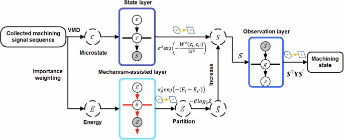
The computation workflow is consistent with Table 2.
To validate the consistency between the established energy feature and generalized wear regularity, the measured wear values are calibrated through Generalized Taylor formula proposed43, which illustrated the relationships of flank wear progression against cutting time under specified working conditions:
$${VB}=C\cdot {t}^{{E}_{t}}{V}_{c}^{{E}_{v}}{f}_{z}^{{E}_{f}}{a}_{p}^{{E}_{{ap}}}{a}_{e}^{{E}_{{ae}}}$$
(17)
Specifically, each experimental group yielded a set of curves fitted by Eq. 17. These calibrated curves served as a comparison with the overall trend of energy feature extracted from corresponding groups in Fig. 3. The variation in segment quantity stems from tool life disparities among cutters, while maintaining an identical time window size.
Fig. 3: The extracted energy indicators and wear values under each milling condition.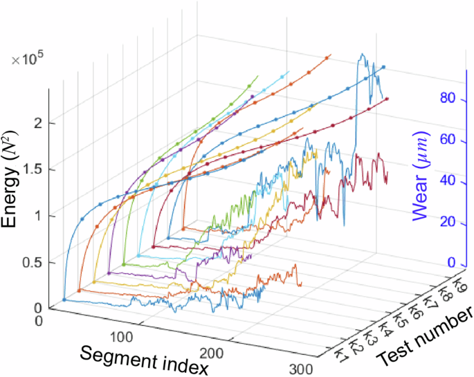
The energies (marker line) and wear values (line) are displayed on the same scales. The y-axis represents 9 different operating conditions, respectively.
The energy indicators effectively reflect the tool wear conditions, and both increase over time, which visually demonstrates an inherent correlation between energy features and physical principles.
Clearly, the cutting conditions have a significant impact on the tool wear rate, leading to different tool state dynamics. Wear occurs significantly faster under conditions of high feed rate and high cutting speed compared to low feed rates and low speeds. This is because increases in feed rate, cutting speed, and cutting depth intensify each cutting cycle, leading to higher cutting forces and elevated temperatures within the cutting zone, which further accelerate tool wear. Specifically, at high feed rates, the coefficient of friction increases, causing localized overheating of the tool surface, material hardening, and potentially leading to impact wear on the cutting edge. Furthermore, tool materials are prone to thermal fatigue during high-speed cutting, which may manifest as crack formation or plastic deformation. Such conditions can further contribute to oxidation, corrosion, and adhesive wear of the tool material. As the cutting depth increases, the volume of material being cut increases, subjecting the tool to greater cutting forces and thermal load. This analysis aids in elucidating how signal features correlate with the wear process.
Before validation, the data under nine operating conditions are preprocessed by applying an 8th-order high-pass filter to remove components below 100 Hz and segmented based on 1-second intervals. The forces in the z-axis were selected as inputs while the tool wear values during the corresponding time intervals were used as outputs. 8 operating conditions were chosen as the training set, with the remaining one serving as the test set, and nine validation trials were conducted.
To compare predictive performance, four statistical metrics were chosen: RMSE, MAE, \({{\rm{R}}}^{2}\), and time. Time refers to the total time taken to model and test the models in a session, automatically recorded by the program.
$${RMSE}=\sqrt{\frac{1}{k}\mathop{\sum }\nolimits_{i=1}^{k}{\left({y}_{i}-{\hat{y}}_{i}\right)}^{2}}$$
(18)
$${MAE}=\frac{1}{k}\mathop{\sum }\limits_{i=1}^{k}\left|{y}_{i}-{\hat{y}}_{i}\right|$$
(19)
$${R}^{2}=1-\frac{\mathop{\sum }\nolimits_{i=1}^{k}{\left({y}_{i}-{\hat{y}}_{i}\right)}^{2}}{\mathop{\sum }\nolimits_{i=1}^{k}{\left({y}_{i}-{\bar{y}}_{i}\right)}^{2}}$$
(20)
Table 2 The proposed algorithm flow
Besides the proposed method, we compared four representative advanced methods, i.e., (Power Spectral Density and Vision Transformer) PSD-CVT18, Stacked Bi-directional Long Short-Term Memory Neural Network with attention mechanism (AT-SBiLSTM)21, Auxiliary Input-enhanced Siamese Neural Network (AISNN)44 and Support Vector Regression Optimized by the Gray Wolf optimization algorithm (GWO-SVR)45. All 5 models are established and tuned to their optimal parameter configurations for optimal performance. Figure 4 presents the prediction results of all models, and Table 3 provides a comparative evaluation of model performance.
Fig. 4: The prediction results of wear by MAGP and 4 compared models in 9 sets.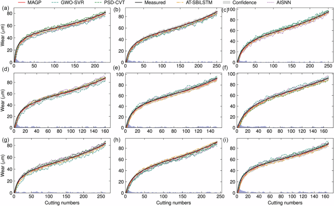
a–i represents 9 groups. Five methods are differentiated using different line styles and color markers, with the gray area representing the confidence interval of MAGP. The cutting numbers in x axis represents signal segment indices.
Table 3 The performance of each model in milling
It can be clearly seen that among several models, MAGP has fewer parameters, with the lowest RMSE. In contrast, PSD-CVT, due to its inclusion of the Transformer architecture, exhibits a significantly higher memory requirement for parameters.
An error-box plot was generated based on the RMSE of the test dataset for each model, as shown in Fig. 5a. Clearly, methods 4 and 5 have high error rates. The RMSE values for methods 2 and 3 are notably similar. The proposed method demonstrates lower error rates in comparison to the other four models. The regression plot shown in Fig. 5c also supports this conclusion, where the predicted values of MAGP have a smaller range and closely follow the measured values.
Fig. 5: The model performance comparations in the milling case.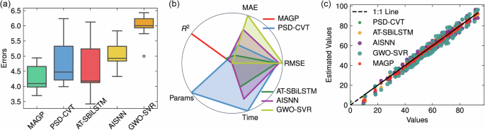
a Box plot of the RMSE values of each model for validation. b Radar plot of the four models. c The regression plot of each model.
To provide a visual analysis, radar charts for the five models were separately plotted as shown in Fig. 5c. The data for these three models were normalized, and the values on the charts were set within the range of [-1, 1]. The axes of the chart represent MAE, RMSE, R2, time and parameters memory. Since lower errors and shorter times are preferable, the model with the smallest area on the radar chart is considered to have the best predictive performance. Clearly, MAGP outperforms the other four models on all error metrics, except for response time, where the performance of GWO-SVR is lower than the other four models. Furthermore, AT-SBiLSTM employs Long Short-Term Memory units and an attention mechanism, greatly enhancing the model’s ability to capture features in sequential relationships. Its features are manually extracted, further increasing its learning efficiency. While AISNN achieves lightweight models and avoids the necessity of manual feature extraction, its use of convolutional layers for automatic feature extraction leads to a slightly longer convergence time compared to AT-SBiLSTM. Compared with other models, it is evident that MAGP exhibits a more balanced performance in terms of lightweight design and generalization.
Figure 6a illustrates the intrinsic mode components of a specific set of cutting force sequences (the 1st group) and the corresponding Hilbert marginal spectrum of this sequence (Fig. 6b). Each spectrum is primarily characterized by multiple peaks, indicating that the frequency components of the force signal are relatively concentrated. At the first few microstates, the frequency is relatively fixed, and these fixed frequencies are related to the periodic action of the tool and the material. As the tool wears down, the frequency gradually spreads out, showing a wider bandwidth. At 75 s and 165 s, there are significant changes in the energy of the force, corresponding to the tool entering the mid-wear and abrupt wear-out stages. As time progresses, there is gradual diffusion in the frequency of the force while the energy shows a gradual increasing trend. This suggests that some new frequencies corresponding to the tool wear emerge during the cutting process, and the intensity of the force increases gradually as the cutting tool wears down. The positive correlation between the intensity and frequency of the force and tool wear implies that it is reasonable to use the energy of the force trend as a feature to assess wear.
Fig. 6: The spectrum and components importance analysis of the milling force sequences.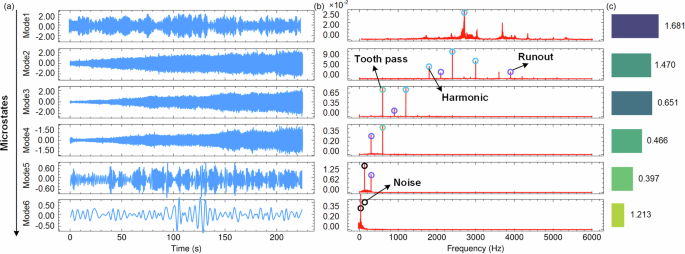
a Microstate-related IMFs; b Hilbert spectrum with significant and negligible frequency components; c MAGP-based feature importance ranking.
Furthermore, in Fig. 7a, we extracted the entropy output established by the state layer and the partition output from the mechanism-assisted layer. Among the 9 data sets, it consistently shows that entropy and partition undergo a similar degradation process, wherein entropy gradually increases while partition exhibits a gradual decrease, particularly evident in the 7 group. The curves show that the trends of entropy and partition features established under condition 9 are essentially consistent (monotonically increasing or decreasing), which aligns with the monotonically irreversible nature of tool wear phenomena. They both progress through three distinct stages of rapid, moderate, and rapid changes, corresponding to the three stages of wear. Particularly, the increase in entropy for group 4 is notably rapid, accompanied by a sharp decrease in partition. In fact, the highest tool wear rate occurs under the conditions of group 4, a change that is also reflected in the partition and entropy features. It can be found that the established entropy and partition features are closely related to the tool wear degradation process.
Fig. 7: The entropy and partition feature analysis in milling.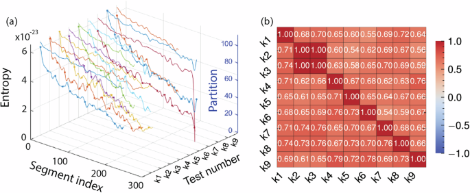
a The extracted entropy and partition in each group. b The feature correlation coefficients between each group, where entropy and partition occupy the upper and lower matrices, respectively.
Indeed, machining process uncertainty can be reflected in the energy distribution of the system. In Fig. 8a, Further short-time Fourier analysis is applied to the force sequences of the 1st groups. In which, wear is divided into three stages: initial wear, steady wear, and severe wear. Through the time-frequency waterfall plot, the characteristic of initial wear is an uneven energy distribution, with larger values at both ends of the frequency band and smaller values in the middle. In the steady wear stage, higher energy amplitudes appear at mid-range frequencies, and the system’s energy becomes more stable overall. In the severe wear stage, the energy at low levels becomes abnormally large, further intensifying the distribution differences and increasing the energy chaos. This observation aligns with the statistical properties of energy presented in Fig. 8b.
Fig. 8: The data information of group 1 and the model hyperparameters in three wear phases.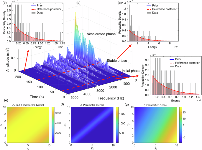
a Full-cycle time-frequency force dynamics; b–d Energy density distributions in three phases; e–g Hyperparameters at each progressive stages.
The energy of microstates at multiple cutting stages was statistically fitted. The statistical forms of energy are shown in Fig. 8b. It can be observed that although both follow an exponential distribution, the prior partition function set to zero deviates significantly from the actual data pattern. This distribution can only sample energy but not the specific microstates, as the combinations of microstates (multi-dimensional IMF) are highly diverse. The Boltzmann distribution defines the forward process of this system, while the Gaussian process model learns the reverse process, inductively deriving the corresponding patterns from the data. The reference posterior partition function output by the mechanism-assisted block closely matches the actual data distribution.
From the perspective of the four kernel hyperparameters in Fig. 8e–g, for \({\sigma }_{p}\)、\(l\)、\(\sigma\) and \(\gamma\), almost without exception, the hyperparameters in the stable stage are closer to larger values. It indicates that the characteristics of the stable wear stage are the most difficult to measure, while the other two stages exhibit more dramatic trends in terms of both entropy and energy.
In fact, during the stable wear stage, due to the absence of new frequency components and impacts from the workpiece or tool during milling, the process exhibits stable entropy and energy. The model requires an increase in hyperparameters to significantly identify subtle changes in features. Specifically, the increased length-scale parameter \(l\) reflects the need for modeling longer-range temporal dependencies during stable wear periods, as the degradation process exhibits smoother transitions compared to the abrupt changes observed in run-in or accelerated wear stages.
Meanwhile, the elevated signal variance \({\sigma }_{p}\) and \(\sigma\) suggest that the model requires stronger regularization to distinguish meaningful wear patterns from inherent system noise when characteristic features become less pronounced. The amplified \(\gamma\) parameter in the kernel further implies that capturing subtle frequency modulations demands enhanced physics resolution.
These adaptive adjustments collectively enable Gaussian process models to maintain high sensitivity to incipient wear progression while resisting false alarms caused by stochastic process variations. From an industrial application perspective, it may provide quantitative guidelines for implementing dynamic hyperparameter optimization strategies that synchronize with different wear phases.
Turning chatter detection
The turning data for validation originates from a public dataset created by Khasawneh46, where 4 distinct stick-out lengths were utilized in the turning process. Three-directional accelerations of both the boring rod and the tool post were recorded during the process. Subsequently, the results of chatter vibration assessments for each segment were tagged. A specific dataset was selected for validation under each stick-out length. The data in this experiment are tagged as four states: stable (S), intermediate chatter (I), chatter (C) and unknown (U). However, as state U does not correspond explicitly to a physical meaning, only S, I and C are selected from which 12 sets are chosen for the validation. The x-axis acceleration signals of the tool post were selected as inputs, with the corresponding vibration states serving as labels, and model validation was conducted.
We compared two advanced methods, i.e., Deep Multilayer Perceptron (DMLP)47, Lightweight Parallel Convolutional Neural Network (LPNN)48, and Wavelet Scattering Network (WSN)49.
Figure 9a–d displays the classification results in the form of a confusion matrix for 3 compared models and our proposed model. As shown in Table 4, the DCNN has a relatively lower number of convolutional layers, resulting in a reduction in the number of parameters. However, this leads to lower recognition accuracy of the model. The WSN, as an application of wavelet transform, can effectively capture the frequency and scale features of signals, as well as provide abstract representations of signals at different levels, which is advantageous for accurately classifying vibration states. The input of LPNN carries some temporal and frequency domain information; however, its model structure has been lightweighted, resulting in its suboptimal performance in vibration state detection. In contrast, the structure of DMLP has limitations that prevent it from adapting well to this classification task, leading to its inferior performance compared to the other models. Table 4 presents the quantitative comparison of the performance of each model.
Fig. 9: The confusion matrices of each model in the turning case.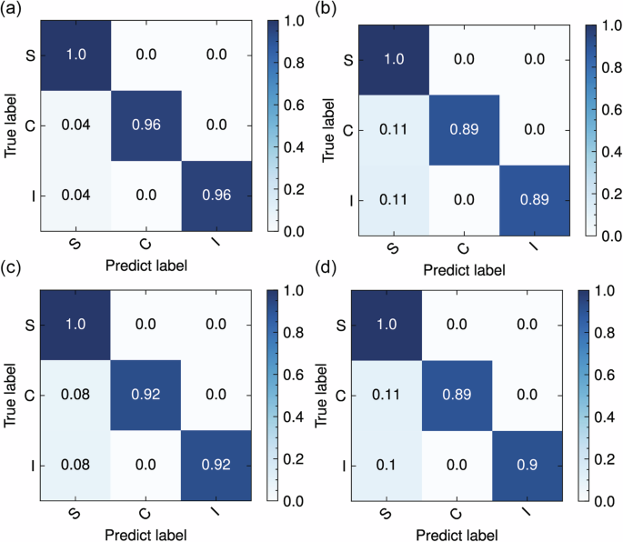
a MAGP b DMLP c LPNN d WSN.
Table 4 The performance of each model in turning
The proposed model achieves a high accuracy of 0.98 and only 0.1522 MB of parameters memory under various processing conditions. This can be attributed to the combination of prior knowledge based on microstates analysis and the GP method, allowing our designed model to achieve significant system fitting ability and sufficient nonlinear mapping ability while maintaining reduced parameters and computational workload. Additionally, the input microstates are segmented to analyze local features more effectively in the time-frequency space.
On the other hand, sequential merging of the time dimension at each level ensures comprehensive extraction of temporal features, thereby enhancing the accuracy of recognizing flutter states. The combination of improved recognition accuracy, reduced parameter count, and enhanced computational efficiency makes our proposed model well-suited for online flutter detection.
Figure 10a displays ROC curves for several different methods, which can be clearly observed the proposed model has the highest accuracy and the lowest false positive rate.
Fig. 10: The model performance comparison.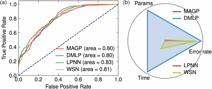
a The ROC curve comparison plot for each model. b The radar plot of each model.
Furthermore, we analyzed feature importance, specifically calculating the mutual information scores between the extracted IMFs and the vibration states. As shown in Fig. 11c, among the 6 IMFs, IMF4 has the highest importance, indicating a comparable conclusion as the Fig. 5. The systematic arrangement of signal characteristics along five dimensions allows for a structured understanding of their individual contributions to the identification of chatter, with those appearing earlier in the ranking likely bearing higher importance in effectively discerning the onset or presence of chatter during machining processes.
Fig. 11: The spectrum and components importance analysis of the turning acceleration sequences.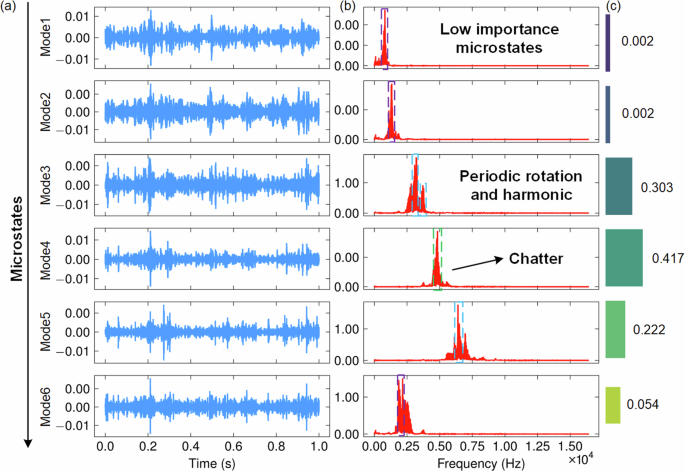
a Microstate-related IMFs; b Hilbert spectrum with significant and negligible frequency components; c MAGP-based feature importance ranking.
This phenomenon can be understood through the frequency components of the acceleration signal. As shown in Fig. 11a, b, the acceleration signal of turning contains a complex mixture of low-frequency and high-frequency components, with the key factor in distinguishing stable states from the other two states being the high-frequency component. The key to distinguishing between chatter (C) and intermediate chatter (I) is the amplitude. Clearly, whether from the high-frequency component or the amplitude in the time domain, IMF4 is the most contributing factor for determining the chatter state, as it simultaneously includes the chatter frequency and has the maximum amplitude relative to other components. It is consistent with the ranking of feature importance and indirectly suggests that it is reasonable to apply importance weighting.
To showcase the consistency between the extracted features and different vibration classes, Fig. 12a plots the 3D bar with entropy and partition for the three classes. Immediate chatter and chatter almost exclusively occur along the path of the approximate exponential curve, indicating that an increase in entropy and a decrease in partition lead to the occurrence of higher vibrations. In Fig. 12b, the scatter plot visualizes the distribution of samples in the 2D feature space spanned by entropy and partition, with marker symbols differentiating three discrete classes. Distinct clustering patterns were observed, where the stable state predominantly occupies low-entropy regions with high partition values. Immediate chatter aggregates in moderate entropy ranges across diverse partition intervals, and chatter localizes to high-entropy domains irrespective of partition metrics. Notably, minimal overlap between stable and chatter suggests entropy serves as a critical discriminator, while immediate chatter exhibits transitional behavior, implying potential hybrid states.
Fig. 12: The sample distribution under established entropy and partition for all sets in turning.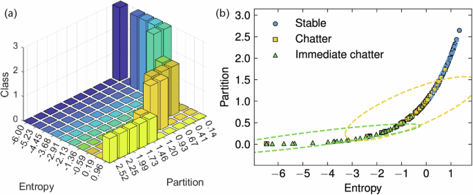
a The 3 d bar of samples classification. b The scatter plot of each sample, where x-axis and y-axis represent the entropy and partition of each group, respectively.
Further short-time Fourier analysis is applied to the acceleration sequences of these two groups. It is evident from the spectrogram in Fig. 13a–c that the substantial values in Fig. 13c are the most prominent, containing more high-frequency components compared to other groups. This alternating high and low-frequency vibration pattern causes drastic energy fluctuations in the spectrum, increasing the system’s uncertainty and resulting in higher entropy values, with converse observation in Fig. 13a. This indicates that the entropy and partition features can directly reflect the state of the processing system over a period and have a stronger correlation than traditional features.
Fig. 13: The data distribution of group 1 and the model hyperparameters in three wear phases.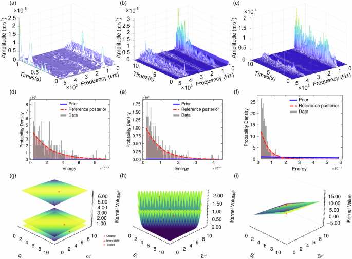
a–c Full-cycle time-frequency force dynamics; d–f Energy density distributions in three phases; g–i Hyperparameters at each progressive stages.
The hyperparameters can reveal the characteristics of different stages of the machining process50. Specifically, the hyperparameters \({\sigma }_{p}\), \(l\), \(\sigma\) and \(\gamma\) play key roles in the entropy of sensor input, energy measurements, and the weighting between physical calculations and data-driven models.
As observed in Fig. 13g–i, in turning vibrations, the stable stage is typically associated with lower frequency changes and smaller vibration amplitudes, resulting in lower entropy values and energy. The model-derived values of \({\sigma }_{p}\), \(l\) and \(\sigma\) are larger, which can be attributed to the model’s ability to avoid amplifying noise when confronted with excessive irrelevant information related to stable frequencies and small amplitudes. As the vibration amplitude increases, the energy also increases, and higher entropy values often indicate that the acceleration exhibits more randomness and complex frequency patterns, causing the three hyperparameters to decrease.
However, an excessively high energy weight could lead the model to focus too much on dramatic changes, overlooking subtle but essential variations in the system. Therefore, the hyperparameter \(\gamma\) balances these two features. In the stable stage, the \(\gamma\) plane of the model has a smaller slope than the other two stages, accompanied by smaller γ values.
Drilling wear identification
The proposed model was validated through a controlled drilling experiment based on the dataset from Verma et al.51. Experiments were conducted on a 3-axis EMCO Concept Mill 105 CNC machine, employing a 9 mm high-speed steel twist drill bit to perforate low-carbon steel workpieces. Machining parameters included three feed rates (4, 8, 12 mm/min) and five cutting speeds (160–200 rpm), generating 15 parameter combinations. Four drill bit conditions were evaluated: flank wear, chisel wear, outer corner wear, and a pristine state. Each condition underwent repetitive single-hole drilling with 8-second vibration recordings per trial. The detailed experiment refers to the Section “Methods”.
We conducted comparative evaluations of the proposed framework against three advanced benchmarks: Kernel-based Self-Training Algorithm with Regularization52 (Kstar), Singular Spectrum Analysis-Bidirectional Long Short-Term Memory network53 (SSA-BLSTM), and XGboost Auto Encoder54 (XGAE).
As illustrated in Fig. 14a, the confusion matrices reveal our model’s classification accuracy with 97% surpassing all counterparts. Kstar possesses an inherent feature dependency that compromises its robustness against tool wear patterns. While SSA-BLSTM effectively decomposes nonstationary signals through singular spectrum analysis, its bidirectional recurrent structure introduces computational bottlenecks during multi-scale temporal feature extraction. The XGAE, despite its powerful feature reconstruction capability, shows limited adaptability to noise-interfered vibration modes due to rigid encoding constraints.
Fig. 14: The confusion matrices of each model in the drilling case.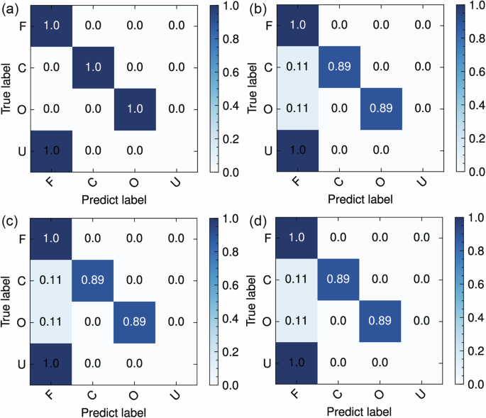
a MAGP b Kstar c SSA-BLSTM d XGAE.
These observations align with ROC curves presented in Fig. 15a, where our model achieves 0.98 AUC, indicative of robust class separation. SSA-BLSTM and XGAE exhibit moderate AUCs with conventional specificity-sensitivity trade-offs. Kstar displays a trajectory with delayed convexity, suggesting latent feature activation emerging only at elevated misclassification risk levels.
Fig. 15: The model performance comparison.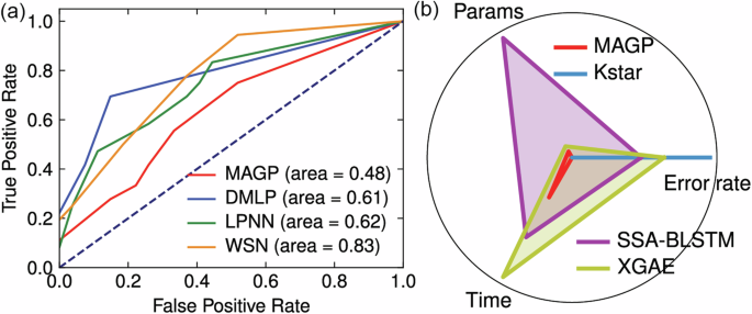
a The ROC curve compared plot for each model. b The radar plot of each model.
The ROC metric quantifies inter-class separability across all thresholds, while the continuous state transitions inherent to turning processes induce gradual feature space overlap, particularly evident in transitional phases between immediate chatter and the other two states. This phenomenon introduces localized interference at decision boundaries, manifesting as an area value of 0.82. However, these metrics remain operationally acceptable given machining monitoring’s tolerance.
The radar chart evaluation in Fig. 15b exposes architectural tradeoffs of each model. The operation of KStar is solely influenced by the feature dimensionality, where the extracted conventional 13-dimensional time-frequency domain features52 facilitate rapid convergence and reduced parameter storage requirements. While the other two models adopt convenient automatic feature extraction approaches, SSA-BLSTM’s bidirectional recurrence and XGAE’s weighting are the crucial computational bottlenecks during model learning. Table 5 presents the specific values of each model’s metric. These results indicate the proposed model can accurately distinguish four wear features without sacrificing computational efficiency.
Table 5 The performance of each model in drilling
The mutual information analysis of an example was conducted in Fig. 16. It identifies IMF 2 and IMF 3 as dominant contributors, correlating with mid-frequency band (250–1000 Hz) energy variations that characterize tool flank wear evolution. Hilbert spectral analysis reveals distinct amplitude modulation patterns: IMF 3 exhibits intermittent bursts during progressive wear, while IMF 2 demonstrates sustained energy accumulation in flank wear.
Fig. 16: The data distribution of group 1 and the model hyperparameters in the drilling case.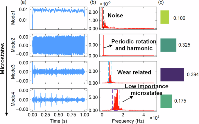
a–c Full-cycle time-frequency force dynamics; d–f Energy density distributions in three phases; g–i Hyperparameters at each progressive stages.
Figure 17a, b present the wear category histograms in the feature space and the sample distributions, respectively. Closely aligned with the turning experiments, distinct state trends and sample clustering characteristics were observed. Entropy-partition mappings in Fig. 17a establish a quantifiable progression trajectory, where tool degradation follows a sigmoidal pattern from low-entropy/high-partition to high-entropy/low-partition. This nonlinear relationship reflects escalating system complexity as tool-edge irregularities amplify vibration stochasticity.
Fig. 17: The samples distribution under established entropy and partition for all sets in drilling.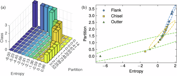
a The 3 d bar of sample classification. b The scatter plot of each sample.
Furthermore, to investigate interdependencies between intrinsic variations within the model and tool state, the time-frequency characteristics of vibration signals under four distinct wear modes and model hyperparameters are provided, with corresponding results illustrating these as detailed in Fig. 18.
Fig. 18: The frequency and erergy information of group 1 in the drilling case.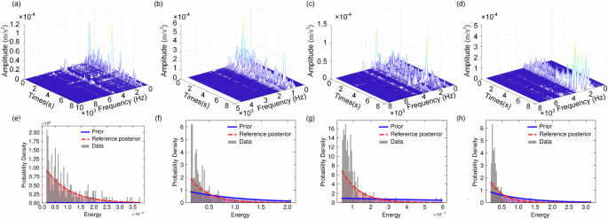
a–d Full-cycle time-frequency force dynamics. e–h Energy density distributions.
The short-time Fourier analysis in Fig. 18a–d confirms different-level enhanced spectral dispersion from the unworn state to other wear states, with dominant frequencies shifting from 2 to 3 kHz. Correspondingly, the distinctions among hyperparameters demonstrate the model’s self-adaptability to varying patterns.
Table 6 presents the hyperparameters of the kernels in four tool states.
Table 6 The kernel space of hyperparameters at each wear state in drilling
For the unworn state, hyperparameters exhibit minimal variability, with elevated \(l\) and reduced \(\sigma\), indicating stable vibration patterns and low disorder. This aligns with the intact tool’s uniform material removal, where acceleration signals exhibit compact probability distributions, reflected in smaller Wasserstein distances.
In flank wear, \(\gamma\) increases significantly, suggesting heightened entropy discrepancies between the data-driven state layer and the mechanism-assisted energy layer. This could also be reflected in the enhanced entropy of the energy distribution.
Chisel wear impacts the tool-workpiece interaction during the initial phase of drilling, whereas vibration signals exhibit steady time-frequency distributions once full workpiece penetration. This characteristic leads to a similar configuration of hyperparameters between non-wear and chisel wear.
Outer corner wear introduces drastic changes in time-frequency and energy distribution due to localized fracture-induced vibrations, which necessitate finer similarity measurements via the Wasserstein kernel and increasing \(\gamma\) against the entropy misalignment of the state layer.
Decreasing \({\sigma }_{p}\) values accommodate rising signal non-stationarity, while \(\gamma\) adjustments ensure the model’s robustness against abrupt wear mode transitions. Notably, the model reduces reliance on data through \(\gamma\) acting as a tunable interface between the data and thermodynamic references, whereas conventional data-driven approaches may typically falter due to insufficient failure-mode samples.