
Materials embeddings, machine learning architectures, and theoretical implementations
Previous research has demonstrated success with partial data models such as gradient boosted trees (GBT), random forests, k-nearest neighbor classifiers, support vector classifiers, and neural networks36. Earlier GBTs were successfully trained by data from22,37.
Following training of the GBT algorithm for topological data, a subsequent analysis demonstrated that electron counts and space groups were the primary distinguishing decision factors to determine material topology22. Model performance was excellent, peaking at 90% for the full GBT model. When the GBT was coupled with ab initio calculations that neglected spin-orbit coupling, accuracy peaked at 92% on the materials with strong confidence in the predicted topological state. As full spin-orbit ab initio calculations enable the direct prediction of material topology, these calculations were not used to supplement the ML models. The primary benefit of using purely structure-based predictions is the encompassing generality, granting an easy method of retraining the models to new situations. Since the original dataset was not accessible, the GBT algorithm without DFT was exactly reconstructed, and applied to the current dataset. On the advanced TQC dataset, it achieved an accuracy of 76% as in Table 3. All algorithms considered are compared to the 76% benchmark, as no additional ab initio calculations were included. In ref. 22, the CGNN was tested, but failed to converge to a reasonable accuracy for topological prediction. Now, it will be seen to have excellent predictive capability.
Four faithful embeddings of the underlying materials are tested. For each embedding, the data format is standardized as follows. Take A to be the set of atoms in the primitive cell. Each atom a ∈ A is associated with two types of information: the atomic identifierva and the atomic positionpa. Finally, the global vectorg is a vector containing primitive cell dimensions and symmetries. Different embeddings are considered for each of the input vectors, and tested over all ML frameworks to determine the best representation.
For a classification with n categories, recall that the one-hot encoding of the i-th category is 0⊕(i−1) ⊕ 1 ⊕ 0⊕(n−i). To enhance generalization over merely using a one-hot embedding of atomic number, the embedding was chosen as \(h(r)\oplus h(c\,(\mathrm{mod}\,\,2))\oplus \lfloor c/2\rfloor\), using the left-step periodic table in Fig. 3 to supply r and c38. This allows generalization over the rows and columns of the periodic table with 7 (rows) + 16 (spinless columns) + 1 (spin slot) = 24 positions per atom. Embedding additional atomic properties was tested, but no additional performance gains were found.
Fig. 3: The left-step periodic table of elements.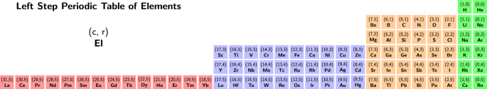
Each atom in the periodic table is labeled with the column and row annotations used for ML.
The position embedding pa is network-dependent, but is stored using fractional units relative to the primitive cell basis. There are two major components of the global data vector g. The first gives the primitive cell dimensions using a sinusoidal encoding39, while the second records the space group with a one-hot embedding. Hyperparameter tuning was used solely for the TQC dataset to demonstrate maximal network performance, and neglected for the remaining tests to demonstrate the ability to immediately generalize.
The full models as described in the methodology are capable of overfitting on any coherent set of training data to an arbitrary extent. Thus, training accuracy is not emphasized. For some tables, previous papers are used as approximate benchmarks for comparison. Since these papers may not use the same dataset, the comparisons are at best indicative.
One implication of the faithfulness of the models is that limits had to be introduced to speed training time. To compare a model to the GBT algorithm, a penalty was assigned to the primitive cells unable to fit in the representation as follows: without knowledge of the underlying input variables, the best predictor of an element in the validation set V is a single label, p, for each element of V. So, this optimal element was used as a default prediction for when materials were too large to use with the ML models. Note that p is extracted from the training set to prevent data contamination. For classification, p is the most common label. For regression, if the loss is root mean squared error (RMSE) or mean absolute error (MAE), then the p which optimizes each of these measures of model error is the mean and median, respectively. This gives a well-defined methodology to compare dissimilar models over an underlying dataset. It also gives a simple baseline model for comparisons, as represented in Tables 1–3.
Table 1 Comparison of ML models for space group and point group one-hot classification problemsTable 2 Comparison of ML models for the categorization problemTable 3 Comparison of ML models for TQCGeneral quantum materials property predictions
The material representations are sufficient to determine the symmetry group. Thus, as a first test of the global power of the ML algorithms, 151,000 materials were taken from the Materials Project and ICSD datasets40,41. The POSCAR file format1 was used as input to supply the ML with atomic types and positions, and the primitive cell basis. The target variable for each material was the space group classification. The symmetry of a material is derived easily from the POSCAR description using structural geometry. Thus, symmetry group classification is perfectly accurate, enabling a verification of the models’ practical implementation.
Two primary implementations for the symmetry groups were tested: the one-hot encodings of the space and point groups. The space groups comprise 230 labels, and the point groups comprise 32 labels. As can be seen from Table 1, ML performance was low compared to analytic techniques. Indeed, this is a known weakness of ML, and is an ongoing area of research in the ML community. The CCNN algorithm did manage to capture the majority of the space symmetries, indicating that spatial relationships are handled best with this direct approach, by comparison with the other three methods.
Formation energy per atom and the magnetic classification were both indexed from ref. 40 for 151,000 materials. Natural errors were expected, due to temperature dependence for experimental results and limited DFT accuracy. Performance on the magnetic dataset was strong, compared to the 81% accuracy on a smaller dataset42. This illustrates the universality of model design as implemented for formation energy (Table 2). However, as expected, classification model performance for regression tasks without modification was weak, which will be improved in the subsequent development.
Topological classification
Three primary sources were used to train the model. The first dataset21 contains a comprehensive list of topological indices for materials. The material information was extracted in the form of POSCAR files from the two largest materials datasets available40,41. For each material, two sets of topological labels were extracted: Ts, a simplified labeling, and Tr, a refinement of Ts. Here, Ts consists of three labels: LCEBR, TI, and SM, while Tr consists of five augmented labels: LCEBR, NLC, SEBR, ES, and ESFD. There are 75, 000 materials with this labeling.
Two requirements were placed on the data. As a first criterion, primitive cells were required to have fewer than 60 atoms. The second criterion arose from the issue that materials are often duplicated by stoichiometric label and symmetry group with minor variations in the POSCAR file. Thus, in cases where the topological labels agreed, the entries were condensed. In cases where there was a discrepancy in the topological data, the material was simply eliminated from the dataset, due to the high probability of a mistaken calculation, or of unusual ambient factors such as temperature and pressure. As an example of this type of situation, 39 tuples of materials were merely minor distortions of each other, distinguished in the ICSD database, but identified in the Materials Project. After the filtration process, 36, 580 materials remained, with 455 datapoints removed. The original dataset evidently contained thousands of duplicate materials. It is worth noting that an ML process based on the original dataset would score artificially higher due to cross-contamination between the training and testing datasets. The topological composition of the dataset is ES, TI, SM, NLC, ESFD with 0.10, 0.27, 0.07, 0.07, and 0.49 as fractions of the whole dataset, respectively.
The majority of model experiments were performed on the TQC dataset. This enabled the diagnosis of specific model issues based on accuracy. Unless otherwise stated, all comments specifically pertain to the full 5 TQC classifications. At the 49% threshold, the model does not necessarily have information transfer between the input and the output, since the most common material type, non-topological, comprises 49% of the dataset. An additional apparent plateau occurs near the 75% accuracy range, after which training is diminished. The CGNN model notably exceeds this threshold. Models were trained on the whole available dataset 20–60 times (epochs) to achieve maximal accuracy on the testing set. All four tested models exhibited an initial fast growth, then an apparent plateau that lasted for approximately one epoch before a more subtle long-term increase in accuracy became apparent. To account for dataset differences, an alternative GBT algorithm was trained for Table 2, based exactly on the specification provided in ref. 22 to compare approaches directly. All the models are either comparable to the GBT baseline, or exceed it, as seen from Table 3.
The optimized implementation for each network is provided in GitHub with notes on optimization. Additional correlation effects were examined, showing weak correspondences between formation energy, magnetic classification, and topological effects in the supplementary material. Ensembles were created to test systemic model errors. Material misclassification was found to happen most frequently for less common elements, especially Pt. Materials with multiple symmetries corresponding to the same stoichiometric formula were more frequently misclassified, unless the topological label was identical for all symmetry phases.
Due to the vast differences in model architecture, ensemble approaches offer a method of enhancing model predictions. As none of the models achieved perfect performance on the testing set, cases where all the models failed to categorize a material’s topological classification properly may be taken as an indication of two potential situations:
The material is accurately represented by DFT, but is misclassified by the neural network (NN)’s due to violating their internal heuristics;
The material itself is miscatalogued due to a deficiency in the DFT computation of the band structure.
As an extension of the model classification, a filtration process is performed. Since the four model archetypes (NNN, CANN, CCNN, CGNN) are capable of achieving greater than 95% accuracy on the training dataset, all four models are trained over several epochs to 95% accuracy on the entire dataset. If the mistakes among the models are uncorrelated, the misclassifications will be uncorrelated, as 36, 580(0.05)4 ~ 0. Any deviation from this scenario demonstrates an interdependence between the models, and allows a model-agnostic method of diagnosing similarities between sources. There were 54 such misclassified materials. Of those materials, CeIn2Ni9, Fe2SnU2, B4Fe (space group 58), and InNi4Tm are positively identified as being topological and likely misclassified due to an insufficient DFT calculations. Additionally, 1:3 and 1:5 compounds are frequent in the misclassifications, corresponding to compounds PtNi3, MoPt3, PdFe3, HfPd3, CrNi3, AlCu3, HgTi3 and HoCu5, GdZn5, EuAg5, CePt5, ThNi5, CeNi5.