
Data
This section outlines our corpus on congressional floor speeches, the annotation procedure used to create the test set for assessing model performance from these data, and the covariates used in the statistical analysis. Section S.3 of the Supplementary Information provides detailed information on the data utilized in this study, including the source, variable descriptions, and descriptive statistics for all variables.
Congressional speeches
We utilize a publicly available Congressional Record scraper and parser33 to extract structured data from HTML files that contain the text of the Congressional Record34. This scraped data includes transcripts of all speeches delivered on the House and Senate floor by Congress Members from 1994—i.e., when the Congressional Record was first digitized—to 2024, as well as each speech’s date and the speaker’s bioguide ID. Each speech was divided into paragraphs (or utterances), resulting in a total of 2,515,806 paragraphs over the sample period. Next, to identify relevant paragraphs for our subsequent analysis, we utilize the ClimateBERT model35 to classify climate and non-climate change paragraphs (see Section S.4 in the Supplementary Information for details). The process resulted in 110,837 relevant paragraphs over the sample period.
Test set annotation
To assess our model performance against a human gold standard, we manually annotated a random sample of 2151 paragraphs from the floor speech dataset using the revised CARDS taxonomy. Given that Democrats are far more likely to discuss climate change in floor speeches, we stratify by party and slightly over-sample Republican speeches. We trained a total of 12 annotators, half of whom contributed substantially to the labeling process. All annotators are or have been research assistants in the Climate and Development Lab at Brown University and have taken a semester-long class on climate obstruction. Additionally, all annotators reviewed the previous CARDS taxonomy and associated video, as well as participated in a lecture and subsequent discussion on the taxonomy updates before starting the labeling process. Each annotator is given one random instance from the climate-relevant paragraphs to label at a time, and each instance is labeled by at least 3 coders. The labeling occurred between October 2023 and February 2024.
As previously noted in Coan et al.21, this is a challenging annotation task even for experts in climate change skepticism. Unsurprisingly, the agreement among the student coders was low—with an overall (pairwise) agreement of 79.8%, marginal reliability based on Krippendorff’s alpha (α = 0.501)—and varied considerably across pairs of coders. To mitigate the challenge of accurately assessing model performance in the face of noisy label data, we had an expert in climate change skepticism and misinformation review instances where there was disagreement among the coders (N = 510 instances) and provided the final label for that instance. Although not completely error-free, this procedure greatly reduced label noise and helped to ensure a more accurate estimate of model performance.
Covariates
Building on past scholarship on interest group influence in Congress36,37 and on the correlates of congressional speech on climate change15, we collected data on a range of covariates at the MoC level. First, we draw on metadata obtained from Congress.gov38 to extract information on the chamber, term, party, age, and state of the MoC associated with each speech. Second, to measure ideology, we use the first dimension of DW-NOMINATE scores provided by Lewis et al.39, which represents legislators’ positions on the dominant ideological dimension in American politics, primarily reflecting liberal-conservative differences on economic and social issues. This dimension explains the largest share of variance in congressional voting behavior and ranges from −1 (most liberal) to +1 (most conservative). Third, we collected data on campaign contributions from the oil and gas industry and the coal mining industry received by the associated MoC of the given speech during the Congress term of the speech. The campaign contribution data comprises contributions from Political Action Committees and individuals associated with each of the three industries. The data was obtained from OpenSecrets’s bulk data40, who derive the data from Federal Election Commission data. The OpenSecrets industry codes we included as part of the fossil fuel industry were: energy production and distribution (E1000), oil and gas (E1100), major (multinational) oil and gas producers (E1110), independent oil and gas producers (E1120), natural gas transmission and distribution (E1140), oilfield service, equipment and exploration (E1150), Petroleum refining and marketing (E1160), gasoline service stations (E1170), fuel oil dealers (E1180), LPG/liquid propane dealers and producers (E1190), and coal mining (E1210). We matched the OpenSecrets bulk data to our congressional speech dataset by matching each member’s Bioguide ID to their corresponding CID (opensecrets_id) in the OpenSecrets data using an existing key41. Finally, we collected district level employment data to capture the economic importance of fossil fuel industries within each member’s constituency from the Bureau of Labor Statistics’ Quarterly Census of Employment and Wages (QCEW). Specifically, we obtained annual employment data for industries classified under specific NAICS codes associated with fossil fuel extraction and related activities: oil and gas extraction (211), coal mining (2121), drilling oil and gas wells (213111), support activities for oil and gas operations (213112), support activities for coal mining (213113), fossil fuel power generation (221112), natural gas distribution (2212), and pipeline transportation (486). The county-level employment data was spatially merged with congressional district boundaries using geographic intersection methods, with employment statistics allocated to districts based on the proportion of county area within each district. We normalize these employment figures by total employment for each constituency (district or state depending on House or Senate member). For more information on the procedure used to build the fossil fuel employment data, see Section S.3 of the Supplementary Information.
Classifying specific contrarian claims
We build on and extend the machine learning framework developed in Coan et al., drawing on recent advances in large language models (LLMs) to overcome several shortcomings of the original CARDS model. First, as made clear in the original Coan et al. study, their model was only appropriate for categorizing contrarian claims within a set of known climate skeptics (e.g., Conservative Think Tanks and Skeptical Blogs). The original model is thus less appropriate for classifying claims when source position is unknown and may produce false positives when classifying non-skeptical content22. Second, the original model relies on multi-class, not multi-label data—i.e., the model assumes the presence of a single category for each paragraph under consideration. This decision proved challenging when dealing with paragraphs containing multiple claims, which is the rule, not the exception. For example, consider the following excerpt:
“And the tragedy is if we were allowed to produce, if this Congress would stop locking up the Outer Continental Shelf, if they would open up the reserves in the Midwest which some of them are taking off in the energy bill, we could have adequate natural gas in this country; the price could be affordable; Americans could be warm; and, the very best jobs in America like petrochemical and polymers and plastic and fertilizer and glass and steel plants and bricks could be made in America, and middle-class working Americans could continue to have the jobs that have historically allowed them to live a quality of life and raise their families.”
The claim that Congress should “stop locking up the Outer Continental Shelf” suggests that fossil fuels are plentiful and should be used (category 7.1.0), while the statement “we could have adequate natural gas in this country” suggests that fossil fuels are necessary to meet energy demand (category 7.3.0). The excerpt also makes claims related to the economy and jobs. Statements that the “the very best jobs in America…could be made in America” as the result of expanding fossil fuel supply suggests that fossil fuels are important for economic growth and development (category 7.2.1), while the text also suggests that current energy bill undermines the ability for “middle-class working Americans [to] continue to have the jobs that have historically allowed them to live a quality of life” implies that policies related to climate change could kill the “very best jobs” (category 4.1.1.2).
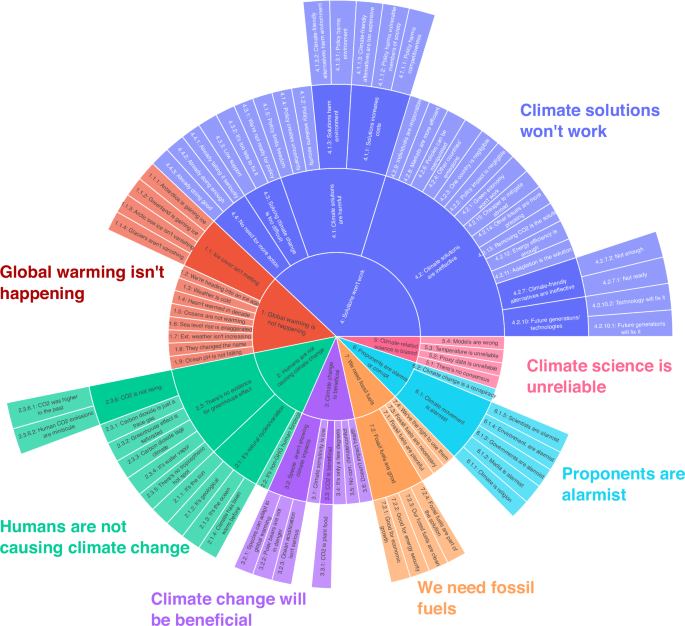
Lastly, though the taxonomy developed in Coan et al. outlines examples of detailed claims challenging climate science and policy solutions, the machine learning model only classifies texts based on 27 level-2 claims. Yet, classifying claims at a granular level is essential for developing an effective response to climate misinformation24, while detailed classifications related to climate solutions allow researchers to more clearly connect specific claims to the general discourses of delay proposed in Lamb et al.’s study3. We address these limitations by developing a multi-label LLM-based framework that classifies texts down to the lowest level of the CARDS taxonomy.
In-context learning with foundation models
The concept of in-context learning (ICL) has emerged as a central paradigm for task adaptation in LLMs42. At the core of this paradigm is the model’s capacity to adapt its behavior based on provided examples, rather than having its internal parameters systematically modified via resource-intensive fine-tuning, which is a notable shift away from traditional machine learning approaches in NLP. ICL leverages the “context“ embedded within the model’s prompt to adapt the LLM to specific downstream tasks, spanning a spectrum from zero-shot learning (where no additional examples are provided) to few-shot learning (where several examples are offered). In essence, LLMs are able to execute an array of tasks by conditioning them on a few examples (few-shot) or task-descriptive instructions (zero-shot). This method of conditioning or “prompting” the LLM can be performed either manually43 or automatically44.
Zero-shot classification. To assess arguably the best case scenario for LLM-based classification performance using ICL, we start by utilizing two frontier models: OpenAI’s GPT4o model and Anthropic’s Claude Sonnet 3.5 model. As of this writing, these models provide near state-of-the-art (SOTA) performance across a range of benchmarks and thus offer a useful baseline for understanding the zero-shot capabilities of large foundation models for classifying contrarian claims.
To utilize an LLM-based approach, we must start by specifying a suitable prompt. We follow current best-practices in the prompt engineering literature45 to iteratively develop the base prompt used in this study (see Section S.5 of the Supplementary Information for the final prompt and a discussion of the prompt development). Our experiments suggest that the use of chain-of-thought (CoT) prompting is particularly helpful for prompt development and classification using foundation models. Zhou et al.46 carried out a systematic evaluation of different chain-of-thought prompt triggers, including human-designed and Automatic Prompt Engineer (APE). In their experiments, allowing the model to break a problem into steps on their own has proven to be more effective than other prompt triggers. For this paper, we utilized the following APE prompt trigger suggested by Zhou et al.46: “Let’s work this out in a step by step way to be sure we have the right answer.”
Dynamic few-shot learning. Research demonstrates that providing examples can allow LLMs to better understand the correlation between the question and the response, thereby improving model performance47. Traditional approaches to few-shot learning augment zero-shot prompts by including a handful of examples for each class, often relying on domain experts to hand-pick specific examples or by randomly selecting from a pool of annotated data. There are practical challenges, however, to implementing the traditional approach, especially for an extensive taxonomy such as CARDS. Providing examples of each claim in Fig. 1 would significantly increase the size of the prompt needed for classification, which will increase the cost and latency of model implementation.
Dynamic few-shot learning extends the traditional few-shot approach by only sending examples that are semantically similar to a user’s input text. This approach utilizes retrieval augmented generation (RAG) to 1) retrieve relevant examples based on calculating the cosine similarity between input text and 2) generate few-shot classifications using the selected examples. Dynamic few-shot learning is particularly useful when one has access to a diverse set of training examples—i.e., either sourced through previous research or by hiring annotators—and may provide the only practical approach to implementing few-shot learning for large, multi-label classification problems.
Fine-tuning scalable alternatives
Although frontier models and in-context learning have been shown to offer competitive performance across a range of classification tasks, these models are expensive to use for large text datasets, thereby making these models difficult to scale in practice (see Section S.7 of the Supplementary Information for a detailed breakdown of costs). Given challenges associated with scaling current SOTA models, we developed a procedure for fine-tuning a smaller, more scalable (i.e., cheaper and faster) alternative.
Fine-tuning data. We start by curating a dataset of high-quality examples for each claim in the revised CARDS taxonomy, aiming for roughly 5 examples per claim. To source examples, we draw on data from the original Coan et al.21 study, focusing on paragraph level data from conservative think tanks (CTTs). When selecting examples, the research team prioritized those that a) effectively captured the claim of interest and b) provided a diverse representation of the ways in which claims are made in real-world texts. We included a carefully selected set of “No claim” examples, again drawing on data from Coan et al.21. Specifically, we select a set of semantically and substantively similar texts that express the opposite view of each claim in the taxonomy. Many of these examples were sourced from quotations and references made to mainstream arguments in CTT text. This procedure resulted in 1691 examples representing the full range of claims in the taxonomy. Note that in addition to using these data for fine-tuning, we also use these examples when carrying out dynamic few-shot learning.
Given that the focus of our analysis is congressional speech, we held out an additional 100 examples from the 2151 manually annotated test set paragraphs to provide additional context on the textual characteristics commonly found in congressional testimonies. OpenAI documentation suggests that we should observe improvements from fine-tuning on 50 to 100 examples, depending on the use case48. Considering the potential difficulties associated with our classification task, we start with the upper-bound of this recommendation. As such, this leaves a total of 2051 out-of-sample paragraphs to assess model performance.
Reverse engineered chain-of-thought prompting. While large foundation models can apply APE straightaway, smaller models must be taught to “reason”. We developed a procedure—reverse engineered chain-of-thought prompting (RECoT)—that uses examples to solve the dual objectives of teaching a scalable model to “reason”, while also training the model to identify specific contrarian claims on climate change. RECoT is carried out in two steps. First, we draw on our fine-tuning dataset and a SOTA model to analyze example text and “reason” through to the final answer provided by the researcher. We explored both Claude 3.5 Sonnet and GPT4o for this step, as these were high performing and affordable options at the time of this analysis. Importantly, the model is instructed to “act” as if it has not been given the correct answers. Second, we then fine-tune a smaller, more scalable base model on the entire CoT responses. After assessing several candidate open- and closed-source base models for RECoT fine-tuning, we found GPT4o-mini provided an effective model for this task, as this model is large enough to efficiently learn from our fine-tuning dataset, but also relatively cheap and fast to ensure model scalability. Supplementary Section S.6 provides a detailed explanation of how we employed the RECoT procedure.
Model performance
Table 3 compares the overall performance of the various modeling approaches described above, classifying claims down to level 3 of the taxonomy (see Fig. 1). Several notable findings emerge from this analysis. First, and somewhat surprisingly, few-shot learning underperforms relative to its zero-shot counterparts. This finding suggests that the procedures used to select suitable context or examples hinder rather than help classification performance. This result is particularly striking given that we use the same examples for fine-tuning with substantially better results.
Second, zero-shot classification with Claude-Sonnet-3.7 (one of the most advanced frontier models at the time of this analysis) delivers remarkable overall performance, consistently achieving the highest scores across our full range of metrics. While this performance is promising, the inference costs for Claude-Sonnet-3.7 are prohibitively high, making this model difficult—if not impossible—to scale to even moderate-sized classification tasks. As demonstrated in Supplementary Section S.7, using Claude-Sonnet-3.7 is nearly 20 times more expensive than GPT-4o-mini and 10 times more expensive than our fine-tuned alternatives.
In light of these scalability constraints, we turn to examining our various fine-tuned alternatives. We took the original fine-tuning dataset with 1691 examples curated from CTTs and generated chain-of-thought responses using both GPT-4o and Claude Sonnet-3.5, creating two distinct datasets. Using GPT-4o-Mini as our base model, we fine-tuned two models—one with each dataset—which we term CARDS-mini-GPT and CARDS-mini-Sonnet. These models demonstrated substantial performance improvements compared to the base model (GPT-4o-Mini): CARDS-mini-GPT achieved a 30.9 percentage point increase in F1-score relative to the 4o-mini baseline, while CARDS-mini-Sonnet achieved a 31.9 percentage point increase. Moreover, incorporating the 100 congressional testimony-specific training examples further enhanced these metrics. The best performing CARDS model (CARDS-mini-Sonnet-2024-12-05) achieved performance metrics that closely approximate (or equal, in the case of Hamming Loss) those of the Claude-Sonnet-3.7 alternative. Crucially, the inference cost is approximately one-tenth the price, making CARDS-mini-Sonnet-2024-12-05 a viable alternative for classifying large volumes of text data.
Statistical methods
To examine the relationship between contrarian claims and key demographic, political, and economic covariates in Congressional speech, we estimated a series of Bayesian mixed effects models. Our unit of analysis is the speech, and the dependent variable of interest is a binary measure for the presence (1) or absence (0) of a contrarian claim in a given speech. While there are several ways to operationalize contrarian speech in our data (each with benefits and drawbacks), our approach captures the adage that it only takes a little dirt to muddy the waters.
Specifically, we examine the correlates of climate change claims using a Bayesian logistic regression model with random effects for legislators and years. Let yit represent whether member of Congress i made a climate change claim during year t. We assume the following probability model:
$${y}_{it} \sim \,{{\rm{Bernoulli}}}\,({p}_{it})$$
(1)
where pit represents the probability that a member of Congress makes a contrarian claim. To model this probability as a function of covariates, we use the logit link function:
$$\,{{\rm{logit}}}({p}_{it})={{\rm{log}}}\,\left(\frac{{p}_{it}}{1-{p}_{it}}\right)={\beta }_{0}+{{\bf{X}}}it{{\boldsymbol{\beta }}}+{\alpha }_{i}+{\gamma }_{t}$$
(2)
where β0 is the global intercept, Xit is a vector of covariates for member i in year t, β is a vector of fixed effect coefficients, αi is a member-specific random intercept, and γt is a year-specific random intercept. The covariates include party affiliation (Republican, Independent), chamber (Senate), sex (Female), standardized age, standardized fossil fuel employment, standardized utility sector presence, and standardized fossil fuel campaign contributions. We estimate the model using Bayesian inference with the following priors:
$${y}_{it} \sim \,{{\rm{Bernoulli}}}\,({p}_{it}) \qquad \qquad {{\rm{(likelihood)}}}$$
(3)
$$\,{{\mbox{logit}}}\,({p}_{it})={\beta }_{0}+{{\bf{X}}}it{{\boldsymbol{\beta }}}+{\alpha }_{i}+{\gamma }_{t}$$
(4)
$${\beta }_{0},{{\boldsymbol{\beta }}} \sim \,{{\mbox{Student-}}}\,t(4,0,2.5) \qquad \qquad {{\rm{(priors)}}}$$
(5)
$${\alpha }_{i} \sim \,{\mbox{Normal}}\,(0,{\sigma }_{\alpha })$$
(6)
$${\gamma }_{t} \sim \,{\mbox{Normal}}\,(0,{\sigma }_{\gamma })$$
(7)
$${\sigma }_{\alpha } \sim {{\mbox{Normal}}}^{+}(0,1)$$
(8)
$${\sigma }_{\gamma } \sim \,{{\rm{Normal}}}\,{t}^{+}(0,.5)$$
(9)
where Student-t+ denotes the half Student’s t distribution constrained to be positive. We use weakly informative priors for all parameters, with Student-t distributions for the fixed effects and half-Student-t distributions for the random effect standard deviations. The model implemented in Stan (http://mc-stan.org) using Hamiltonian Monte Carlo with 4 chains, each with 3000 iterations (including 1000 warm-up iterations).