
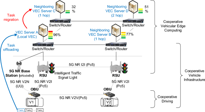
The simulation platform uses Intel Core i7-8655U CPU processorwith a maximum frequency of 4.60 GHz. We constructed 21 cooperative VEC servers using the Matlab simulator (i.e., a local VEC serve and 20 neighboring edge servers connected to the local server within 3 hop counts, as shown in Fig. 5), and each server was deployed at a distance of 1 km from its neighboring server. These servers are interconnected via optical fiber links. Related information (RI) packets are broadcast in a flooding manner in 3 hop counts to awareness state of neighboring servers. In an overall VEC network (e.g., city environment), any local VEC server can operate MCATM to migrate tasks to its neighboring server. VEC servers can be set up at intersections, road sections, or locations in the road network where they are needed. Considering the efficiency of network information exchange, path search tree, and packet communication latency, we recommend that local VEC servers do not connect too many neighboring servers. We also do not recommend generating RI packets at high frequency to avoid broadcast storm, despite their potential benefit in enhancing the awareness of neighboring VEC conditions.
Fig. 5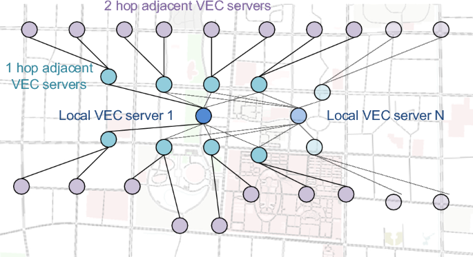
Example of VEC network topology.
We sue 3 metrics to analyze system performance. The delay metrics include the transmission delay, execution delay, and propagation delay, which depend on the simulated scenario. Note that execution delay is the time at which the task is executed on a local or neighboring server. The success rate metric is defined as the percentage of tasks successfully migrated to a neighboring VEC server. The success rate is obtained by dividing the number of task migrations by the total number of tasks (i.e., success rate = migrated tasks / total tasks). It is used to observe the probability of successful task migrations. The elapsed time metric is the run time of the algorithm in the real system, which is directly obtained from the system on the testing platform. The CPU frequence of the testbed affects the elapsed time. The faster the CPU speed, the shorter the time required to execute the algorithms.
In the context of the simulated VEC network topology, 172 packets are transmitted throughout the VEC network when the RI packet generation is set to 10 Hz. It takes 0.00344 s for total transmission, as shown in Fig. 6. As the frequency of RI packet generation increases, the network cost. In this figure, when the RI packet generation reaches 50 Hz, the number of packets and transmission time increase from 1720 and 0.00344 s to 8600 and 0.0172 s, respectively. Maintaining the same architecture but increasing the number of servers to 60 in the VEC network, as shown in Fig. 6, leads to an increase in the number of packets and transmission time, reaching 25,800 and 0.0516 s, respectively. Consequently, as the frequency increases, the number of packets and transmission time increase accordingly.
Fig. 6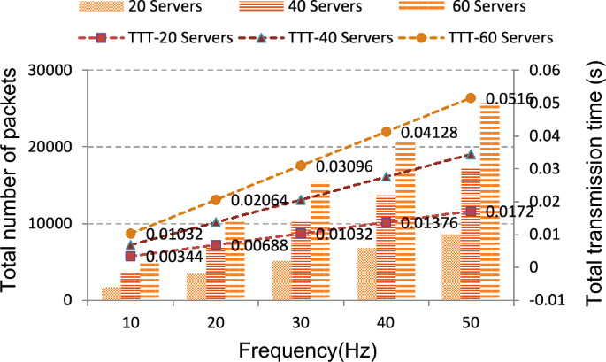
Analysis of the VEC network.
We set data rates of 309.1 Mbps and 618.1 Mbps as calculated by 5G New Radio Frequency Ranges 1 for the Uu interface according to41 when the maximum resource block allocation in 5G NR is set to 135 and 270, respectively. The data transmission rate is influenced by numerous factors, including the ratio of time slots in data transmission, the network environment, the number of online users, and the processing capabilities of the sender and receivers. Table 7. provides additional simulation parameters.
Table 7 Simulation parameters.
We performed a comprehensive comparison of our scheme against the following baselines:
Adjustable analytic hierarchy process37 (AAHP)
The AAHP employs a similar approach to select the target server for task migration, with the ability to adjust its weight matrix for the previous decision.
Dijkstra40
Dijkstra’s algorithm is a method for finding the shortest paths between nodes in a weighted graph. It is commonly used to determine the shortest path from a source node to all other nodes.
Open Shortest Path First (OSPF)42,43 is a link-state routing protocol utilized by every node within a network. The fundamental concept of OSPF is that each node maintains a table or map of its connectivity to the network. Each node then independently calculates the shortest routing path to every possible destination in the network using Dijkstra’s algorithm. If multiple paths with the same cost exist to a given destination, tasks can be allocated to these paths.
Resource allocation of task offloading in single hops (RATOS) and Resource allocation of task offloading in multiple hops (RATOM)
These two methods share similarities with MCATM in terms of task allocation. They utilize the AAHP to select the appropriate VEC server either in one or multiple-hop neighbors. Both RATOS and RATOM subsequently employ the Dijkstra algorithm to identify the shortest path between the source and destination.
Optimal enumeration service deployment algorithm (OESDA)30
OESDA enumerates all collaborative resource configuration schemes involving m servers and calculates the average response delay. By comparing all average request response delays, the optimal configuration scheme can be obtained. In our simulation, OESDA evenly distributed the unprocessed tasks to neighboring edge servers. Tasks are transmitted to 1 hop edge server, and OESDA sequentially routes tasks to neighboring edge servers, starting from the closest one. If the collaborative resources of the edge network cannot meet the task requirements, the task is routed to the remote cloud computing center for processing.
Lyapunov-guided soft actor-critic (SAC) algorithm (LySAC)33
LySAC is a Lyapunov-guided DRL method that includes the state, action and reward, then adopt the soft actor-critic (SAC) algorithm to learn the optimal resource allocation. The architecture of the LySAC algorithm includes an actor network, two critic networks and two target critic networks, all of which are the deep neural network (DNN). The specific model training of LySAC is required before testing. We adopt the same parameter settings and adjust the relevant parameters according to the scenario described in this paper. Each vehicle will generate 5 different tasks in any timeslot and offloads them to the VEC server for computation. Figure 7 shows the reward curve of the training stage for different numbers of vehicles. We can see that the learning curves for different numbers of vehicles first increase, then decrease. In this scenario, since the network topology is not complex, thus, the VEC server can quickly reach to a stable state after quick learning (approximately after 700 episodes) when the number of vehicles is 10 or 20. When we set 30 vehicles in this training stage, its reward value increases slowly to a stable value. This is because the VEC server first learns the policy to maximize the reward and guarantee the low-latency constraint, thus the learning curve first increases. Afterwards, the VEC will eventually learns an optimal policy to maximize the reward while satisfying its constraints, therefore the learning curve finally becomes stable. We can also see that the rewards have some jitters after reaching stability, because the VEC server remains in a stochastic environment due to the random task arrival, which affects the learning of the VEC server.
Fig. 7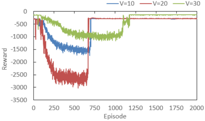
In the testing stage, the LysAC using the optimal model established in the learning stage. Based on our observation and simulation analysis, LySAC should perform at least 100 episodes to obtain the lowest delay. Therefore, during the testing stage, each simulation was set to be executed 100 episodes per round, and the average value was obtained after 30 rounds. The results are presented in Fig. 8. In Fig. 8, when the edge server is busy, i.e., capability = 20%, It may not have sufficient capability to handle tasks, thus its average delay for executing various task volumes (10 to 50 tasks generated by each vehicle at one timeslot) is relatively high. As the server capability increases, more computing resources can be provided for computing tasks, resulting in a decrease in the average delay. In general, with the same capability, the average delay will increase slightly with increasing task volume.
Fig. 8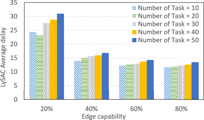
LySAC average delay under 100 episodes.
To understand the operational status of LysAC, we conducted various simulations in the testing stage. Figure 9 shows the delay curve of 50 tasks over 100 episodes. In this scenario, LysAC has already completed its model learning, so the delay is not much jitter as in learning stage. When the edge server has only 20% available capability, the delay jitter is greater. This occurs because the server may not have sufficient capability to handle tasks in this scenario, thus tasks may be queued in the buffer. As the capability increased, we observed that the delay jitter is relatively minor. When server’s capability = 80%, the delay only slightly jitters.
Fig. 9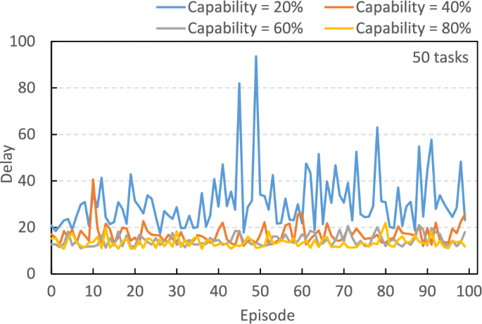
Delay curve of LySAC in the testing stage under 100 episodes.
Comparison of the server selection mechanism
The weight matrix of the AAHP will be adjusted based on previous decision outcomes to prevent the repeated selection of a single MEC server. However, the AAHP algorithm employs a single-layer decision strategy, which may limit its ability to adaptively modify the weight matrix due to its small amplitude. In contrast, the WVAHP utilizes a two-layer decision-making approach, effectively addressing the shortcomings of the AAHP. This section compares the WVAHP and AAHP algorithms under identical conditions as evaluation criteria and calculates the standard deviation of task allocation across all MEC servers. Given that all MEC servers share the same service resource capacity constraints, a smaller allocation standard deviation indicates a more balanced load among the MEC servers and a more effective resource allocation.
Here, we perform the simulation of 50 times in the same scenario to observe the selection counts of the servers. Every 10 simulations were grouped together to calculate the standard deviation of the server selections. During these simulations, we varied the number of tasks from 20 to 50 (denoted as num = 20,…,50), with every task randomly generated by a server. The primary objective of the WVAHP is to balance resource allocation for task migration, with a preference for server selection counts that closely match those of others.
In Fig. 10 (a), we observe that WVAHP and AAHP methods produce similar standard deviation values when the number of tasks is less than 30. The processing capabilities of the servers exceed the task requirement, idle server states result. However, it is worth noting that in each group, the standard deviation values for the WVAHP are consistently lower than those for the AAHP. This validates the effectiveness of the WVAHP in evenly allocating tasks to appropriate servers, thereby achieving better load balance than the AAHP. Figure 10 (b) to 6(e) depicts the standard deviation with error bars for the scenarios with various numbers of tasks. Basically, both WVAHP and AAHP have reasonable errors, which can be observed from Fig. 10 (b) to Fig. 10 (e). Furthermore, in Fig. 10 (e), we can see that the WVAHP model exhibits more uniform allocation than AAHP in the scenario of large number of tasks.
Fig. 10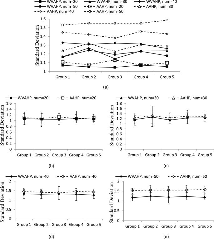
Standard deviation of the selected count.
Comparison of path selection algorithms
As illustrated in Fig. 11, the PACB algorithm consistently achieves lower migration delays than the Dijkstra algorithm in both scenarios. The migration delay tends to increase with an increasing number of tasks, which is a logical outcome. More tasks transmitted in the network consume network resources, which increases migration costs. In Fig. 11 (a), three overlapping trend lines are the Dijkstra algorithm in terms of the average delay, maximum delay, and minimum delay. These lines exhibit varying growth rates as the number of tasks increases. This behavior is due to the Dijkstra algorithm consistently selecting the same path for task transmission, resulting in heightened transmission and propagation delays, as evident in both Fig. 11 (a) and (b). The primary feature of OSPF uses distributed link-state protocol. When the status of a link changes, OSPF employs a flooding method to disseminate this information to all adjacent nodes. As a result, OSPF can quickly find the shortest path. Additionally, OSPF is similar to the PACA method, as it can allocate traffic to multiple shortest paths. Generally speaking, OSPF exhibits slightly lower average, maximum, and minimum delays compared to PACA. As illustrated in Fig. 11(a), the average delay of OSPF is less than that of PACA; Fig. 11(b) further demonstrates that OSPF’s average delay is predominantly lower than that of PACA. However, OSPF has several drawbacks. The frequent exchange of link state information between nodes requires all nodes to establish a link state table, which essentially serves as a global topology diagram. As the network scale increases, the maintenance costs of the link state database also rise. Additionally, OSPF only considers path overhead when calculating the shortest path, without taking into account other factors such as bandwidth utilization and network congestion.
Fig. 11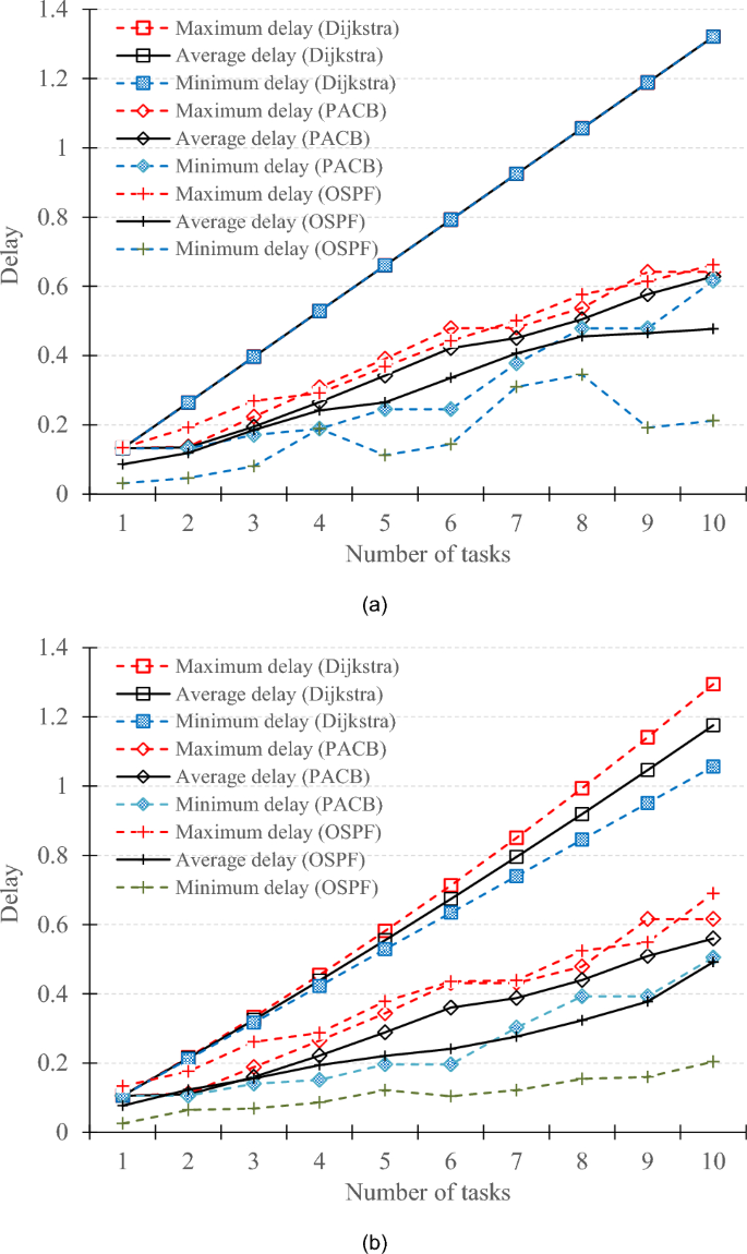
Comparison of task delays under (a) fixed task size (500 kb), and (b) various task size (400 ~ 500 kb).
Link utilization refers to the utilization rate of the overall network communication capability, which is calculated as the proportion of the total number of links in the task migration path divided by the total number of links in the overall network, i.e., link utilization = number of links in the migration path / number of links in the overall network. Figure 12 compares the link utilization of the PACB and Dijkstra algorithms. Because the PACB algorithm selects multiple transmission paths, it uses more communication links than Dijkstra’s algorithm’s single-path transmission, resulting in higher link utilization rates under simulated rounds. Through calculation, the PACB algorithm has an average call rate improvement of 34.09% compared to Dijkstra’s algorithm, which can better use the limited communication capacity of the network. Since OSPF updates link status in real time, it can consistently identify the shortest path. According to the OSPF algorithm, the transmission time of routing paths increases when a task is allocated to a specific transmission path. Consequently, other tasks will be assigned to alternative suitable routes to prevent the problem of scheduling all tasks on the same path. As a result, OSPF exhibits higher link utilization compared to Dijkstra’s algorithm. Furthermore, the PACB algorithm allocates all tasks across the entire network, leading to slightly higher link utilization than that of the OSPF algorithm, as illustrated in Fig. 12.
Fig. 12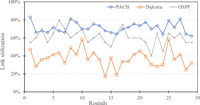
Comparison of link utilization.
Comparison of task migration costs
To assess the overall migration cost of networks, we aggregated the delay of each task, resulting in a total delay. This allows us to analyze and compare the efficiency of our proposed MCATM with that of other resource allocation methods. The target server in the RATOS algorithm only considers servers within a 1-hop range, which causes latency to increase rapidly as task volume rises. In contrast, the MCATM algorithm and RATOM algorithm consider MEC servers within N-hop range as potential candidates. When neighboring servers are occupied, there is a high probability of finding the most suitable server among these candidates. Furthermore, although both the MCATM and RATOM algorithms are based on Dijkstra’s algorithm, the MCATM algorithm takes into account the mutual influence between computing tasks and the dynamic changes in transmission path weight values. This approach reduces the allocation of computing tasks to redundant paths and maximizes the communication capabilities of the entire network. Consequently, the transmission latency of the MCATM algorithm is expected to be lower than that of the RATOM algorithm.
Figure 13 presents the task total delay comparisons under various service capabilities, ranging from 20 to 80%. In most scenarios, MCATM results in task total delays that are either equal to or lower than those of other approaches. This is because MCATM considers additional servers for task migration when the neighboring server is at full capacity. Consequently, it enables faster execution of computational tasks, thereby avoiding the need to wait for neighboring server CPU resources.
Fig. 13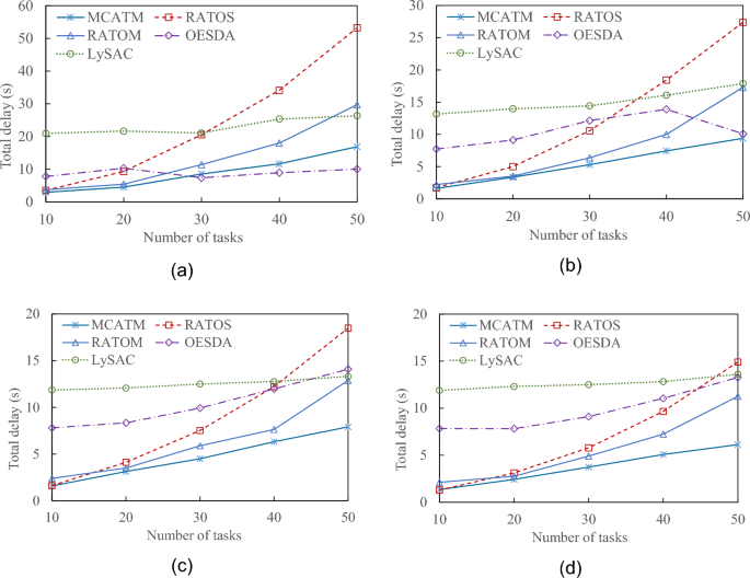
Comparison of total delay of task computations under server service capabilities of (a) 20%, (b) 40%, (c) 60%, and (d) 80%.
In the OESDA method, a VEC server selects the nearest neighbor for task migration, regardless of whether the nearest neighbor is the best choice. This is the primary reason why OESDA generally results in larger total delays than RATOS, as indicated in Fig. 13 (c) and (d). However, when the server capabilities are below 40%, as shown in Fig. 13 (a) and (b), OESDA appears to outperform RATOS. In the OESDA method, if 1-hop neighboring servers cannot handle the substantial task load, tasks are transmitted to the cloud for execution. Assuming that a cloud server has ample computing capability, the execution time in the cloud can be neglected, and the task transmission time between the edge server and the cloud is set at 0.2 s 44. This explains why OESDA achieves lower total delays than the other methods when the number of tasks exceeds 30 and server capabilities remain at 20% (refer to Fig. 13 (a)). In this scenario, the OESDA offloads some tasks to the cloud, which reduces to a reduction in the total task delay.
During the testing stage, LySAC can find a good solution with fewer episodes. However, based on our previous analysis, it is recommended to perform it at least 100 episodes, and it also increases the delay, as shown in Fig. 12. If LySAC performs only 10 episodes, its total delay will be lower than that of MCATM. Nevertheless, its solution that was found in 10 episodes may not be the best one. Because LySAC executed 100 episodes, it has a higher total delay than MCATM.
Despite RATOM considering n-hop neighbors’ available computing resources, similar to MCATM, it experiences higher total delays than the proposed MCATM. Even when RATOM selects the same server as MCATM, its task migration is likely to be transmitted along the same network path, leading to task congestion on that path. In contrast, MCATM, which prioritizes network load balancing, evenly distributes migrated tasks across different paths. Consequently, MCATM achieves lower total delays than the other methods.
The total delay for each approach increased as the number of tasks increased. However, the MCATM growth curves show a slower rate of increase than those of the other methods. Furthermore, as the server service capability increases (as shown in Fig. 13 (a) to (d)), the total delay increases for each approach.
Figure 14 compares the average task delays across different server service capability scenarios, ranging from 10 to 90%, with the number of tasks set to 20–50. The average delay in MCATM remains low across various service capability scenarios, primarily because tasks are efficiently migrated among n-hop neighbors. As the service capability gradually decreases, the average delay also increases. Due to the limited computational resources in n-hop VEC servers, they cannot satisfy the demands of all tasks. Consequently, the network becomes overloaded, resulting in a significant increase in the average delay.
Fig. 14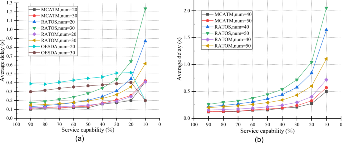
Comparison of the average delay.
For each mechanism (MCATM, RATOS, RATOM, and OESDA) with varying numbers of tasks (num = 20–50), the average delays also increase accordingly. The OESDA lacks optimization for task migration path selection which generally results in poor performance. However, in the 10% service capability scenario, OESDA’s average delay is notably reduced. This is because OESDA offloads tasks to the cloud when local computational resources cannot meet the task requirements. Nevertheless, this is an exceptional case, because overloading cloud services can occur when many tasks are sent to the cloud, which requires careful consideration. In scenarios where the server service capability is low, the average delays for all mechanisms tend to increase. Compared with the other methods, the MCATM’s delay curve shows a slower rate of increase.
In the simulation, when the average response time of a computing task is less than the maximum tolerable delay, the migration of the computing task to a suitable MEC server can be considered as successful. Theoretically, the success rate of task migration should decrease as the service capability of the server decreases, and it should also decline with an increase in the number of computing tasks. In Fig. 15 (a) and (b), we observe a decreasing success rate as the server service capability increases. The OESDA method consistently achieves a 100% success rate for task execution due to cloud service server assistance, it is not considered in the comparison. When server service capability is high, tasks can easily find suitable servers for migration. As the service capability decreases and the number of task increases, all the schemes exhibit a decreasing success rate. Compared to the other schemes, RATOS consistently achieves lower success rates across all scenarios (num = 20–50 tasks). Its success rate rapidly declines when service capability falls below 60%.
Fig. 15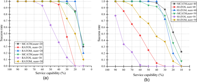
Success rate of task migration.
RATOM and MCATM outperform better than the RATOS baselines do, primarily due to their task cooperative strategies involving n-hop servers. Compared to RATOS, RATOM, which benefits from n-hop server assistance, achieves higher success rates. In Fig. 15 (a), for num = 20, MCATM maintains a 100% success rate even when the service capability is less than 20%. For num = 30, MCATM achieves a success rate of over 80%. Even in Fig. 15 (b), for num = 40 and 50, MCATM maintains success rates of approximately 88% and 77%, respectively, in scenarios where service capability remains at 30%. By comparing the success rates between Fig. 15 (a) and (b), we conclude that MCATM can effectively handle 50 tasks while maintaining a satisfactory success rate.
The MCATM consistently achieves a higher success rate than the other mechanisms in every aspect. Despite RATOM’s attempt to find an appropriate server within multi-hop neighboring servers, its success rates generally fall short of MCATM’s performance under most conditions. This is primarily due to the RATOM’s lack of an optimized configuration scheme to prevent duplicate selection of the same server.
Comparison of the algorithm elapsed time
MCATM can effectively utilize the computing power of neighboring servers to meet the constraints of computing tasks and achieve migration services. In theory, more neighboring servers can provide more computing power. However, when examining the latency caused by transmission distance and packet forwarding, servers that are too far away may not be able to meet the time constraints of computing tasks. In addition, calculating WVAHP will also increase its running time as the number of candidate servers increases. Figure 16 shows the comparison of running time between MCATM and LySAC. There are a total of 5 vehicles in this simulation, each generating multiple tasks at the same time, such as randomly generating 5–15 tasks. Each simulation is executed 30 times, and the average value is taken as shown in Fig. 16. Using the MCATM method, when the local server has 5 neighboring servers, it takes approximately 0.041221133 s to process 25–75 tasks (5 vehicles, task = 5–15); The computation for processing 275 ~ 325 tasks (5 vehicles, task = 55 ~ 65) takes approximately 0.0907817 s. Please note that this eclipse time is only the operating time of these two methods and does not include task offloading, migration, computing, and other times.
Fig. 16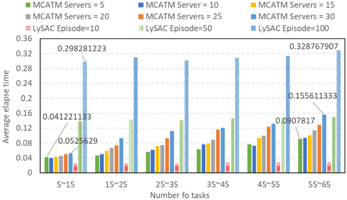
Comparison of the elapse time.
As the number of neighboring server increases, the eclipse time required for the same number of tasks does not decrease. This is because increasing the number of servers requires MCATM to perform more dimensional calculations, which results in a slight increase in eclipse time. When there are 30 neighboring servers on the local server, it takes approximately 0.0525629 s to process the computation of 25–75 tasks (5 vehicles, task = 5–15). Although it adds a bit of time, neighboring servers can assist local servers by handling several times the amount of computing tasks.
The disadvantage of LysAC is that it requires a significant amount of time in the learning stage. However, during the testing stage, it can quickly load its learning model and find suitable solutions in a few episodes. Figure 15 shows the time consumption of LySAC for executing 10, 50, and 100 episodes in the testing stage. When executing 10 episodes, 25 ~ 75 tasks and 275 ~ 325 tasks only require 0.025599773 s and 0.027847707 s, respectively. When it executes 50 episodes, 25 ~ 75 tasks and 275 ~ 325 tasks require 0.138937897 s and 0.150185093 s, respectively. According to the simulation, the episode has a significant impact on the collapse time of LysAC. When it executes 100 episodes, 25 ~ 75 tasks and 275 ~ 325 tasks require 0.298281223 s and 0.328767907 s, respectively. Although LysAC can find the best solution in 100 episodes, it requires more eclipse time than MCATM.