Functional hierarchy of the human neocortex across the lifespan

Materials

The individuals in the study were selected from five imaging datasets: the BCP49, the development, young-adult and ageing cohorts of the Human Connectome Project (HCP-D, HCP-YA and HCP-A, respectively)50 and the Healthy Brain Network (HBN) dataset51. Individuals in the BCP ranged from 16 days to 6 years old, with 557 individuals scanned at 1,095 unique time points before gradient-based quality control. We initially used 652 individuals (age 5.6–21.9 years) from HCP-D, 1,206 individuals (age 22–37 years) from HCP-YA, 725 individuals (age 36–100 years) from HCP-A and 772 individuals from the HBN (age 5.6–21.9 years). Across all five cohorts, our dataset included 3,912 individuals.

Ethics

All data were obtained from publicly available studies (BCP, HCP-D, HCP-YA, HCP-A and HBN). Each contributing study received ethics approval from its local institutional review board and obtained informed consent (and assent where appropriate). The present work analysed de-identified data and complied with all relevant data use agreements.

Quality control

We excluded infant data with excessive motion, cutting the BCP dataset from 557 individuals with 1,095 time points to 343 individuals with 760 time points. For the entire lifespan dataset, we used visual and clustering-based gradient quality control, excluding problematic gradients from the main analysis. Using this procedure, we excluded one additional data point from the BCP for a total of 759 time points and 343 individuals (158 male individuals, 176 female individuals and 9 unreported). We excluded 2 sets of gradients from the HCP-D for a total of 650 individuals (301 male individuals and 349 female individuals). We excluded 2 individuals from the HBN dataset for a total of 770 individuals (458 male individuals, 275 female individuals and 37 unreported). Preprocessing-related failures (for example, unsuccessful surface reconstruction or unusable resting-state fMRI data) led to the exclusion of 88 HCP-YA participants. Visual inspection and k-means clustering of Procrustes-aligned gradients identified an additional 50 corrupted gradient sets, yielding a final HCP-YA sample of 1,068 participants (482 male and 586 female). We excluded no data from the HCP-A (725 individuals; 319 male and 406 female). These decisions were justified by examining individual gradients as well as their associated metrics (dispersion, range and similarity to template) in combination with k-means clustering applied to the set of all individual gradients. In total, our final analysis included 3,972 unique gradient sets from 3,556 individuals. Supplementary Fig. 3 shows the distribution of participants’ ages by cohort after quality control. Cohort-wise median mean Power’s frame-wise displacement (FD) after quality control is shown in Supplementary Table 3.

fMRI preprocessing

We used an rs-fMRI preprocessing pipeline that is consistent with the HCP52. The preprocessing pipeline includes (1) head motion correction using FMRIB Software Library (FSL) mcflirt; (2) echo-planar imaging (EPI) distortion correction using FSL topup to generate distortion correction deformation fields using a pair of reverse phase-encoded field maps (that is, anterior–posterior and posterior–anterior or left–right and right–left); (3) rigid (six degrees of freedom) registration of a single-band reference (SBref) image to field maps; (4) rigid boundary-based registration (BBR) of distortion correcting the SBref image to the corresponding T1-weighted (T1w) images, with pre-alignment using a mutual information cost function; and (5) one-step sampling using combined deformation fields and translation matrices, producing motion- and distortion-corrected fMRI data in each individual’s native space (T1w space).

We denoised the fMRI data before further analysis. First, we detrended the data by high-pass filtering with a cut-off frequency of 0.001 Hz to remove slow signal drift. Next, we used independent component analysis based automatic removal of motion artefacts (ICA-AROMA) denoising53 to remove any residual motion artefacts. This involved performing a 150-component ICA on the fMRI data and classifying each component as either BOLD signal or artefact on the basis of high-frequency contents, correlation with realignment parameters from head motion correction, edge effects and cerebrospinal fluid fractions. Independent components classified as artefacts are (aggressively) removed by regression.

Structural and diffusion preprocessing

Structural data underwent automated quality assessment54,55, inhomogeneity correction and linear transformation of T2w images to the respective T1w images. We then delineated white matter, grey matter and the cerebrospinal fluid with automated segmentation (Supplementary Figs. 14 and 15). Usable diffusion data selected using a deep-learning-based semi-automated QC56 were corrected for signal drop-out, pile-up and eddy-current and susceptibility-induced distortions57. Co-registration between diffusion MRI (dMRI) and structural MRI (sMRI) using multi-channel nonlinear registration was performed with the symmetric normalization method available in Advanced Normalization Tools (ANTs)58. Finally, manual visual inspections were done to ensure quality.

To establish a consistent coordinate system across the entire lifespan, we used in-house lifespan surface atlases extended from a previous study59. The reconstructed cortical surfaces of each individual were first registered to age-matched cortical surface atlases for vertex-wise correspondence among all the surfaces across the lifespan (Supplementary Fig. 14). Cortical surfaces were mapped onto a unit sphere and Spherical Demons60 was used to perform registration between the spherical surfaces of the individuals and the age-matched surface atlases. The vertex-wise correspondence established as a result of spherical registration was then propagated to the white and pial surfaces using one-to-one correspondence between the spherical and standard representations of the white and pial surfaces. Cortical surfaces used in the analysis comprised 20,484 vertices including the medial wall and 18,644 vertices excluding the medial wall.

Structural and diffusion indices were computed in the same manner for all cohorts. Specifically, cortical thickness is defined as the Euclidean distance between two correspondent vertices on the white and pial surfaces and myelination is quantified using the ratio between T1w and T2w images41. Spherical mean spectrum imaging (SMSI)61,62 was used to calculate intracellular volume fraction, extracellular volume fraction, intrasoma volume fraction, microscopic fractional anisotropy, microscopic mean diffusivity, microscopic anisotropy index and orientation coherence index. The diffusion tensor model was used to calculate fractional anisotropy and mean diffusivity.

Functional gradients

FC matrices were computed from the vertex-wise fMRI time series for each acquisition from each individual using the pairwise Pearson correlation coefficient. For individuals with repeated scans (BCP participants), acquisitions were grouped by time point, and we averaged FC matrices within each time point. We then subjected each mean FC matrix to row-wise thresholding (top 10% of connections retained), and computed the normalized angle matrix, in keeping with previous gradient literature1,14,63,64. Mean FC degree was computed for each individual as the average across vertices of the sum FC weights in the individual’s thresholded mean FC matrix. We computed ten FC gradients for each individual using the diffusion embedding implementation in BrainSpace64, with the normalized angle matrix as the input affinity matrix. To align individual-specific gradient axes consistently across the lifespan, we computed a set of ‘template gradients’ through weighted principal component analysis (WPCA) of all individuals’ gradients. We began by applying a controlled nonlinear transformation to each individual’s age, taking the square root of age to capture rapid changes in early life. The transformed ages were partitioned into ten equally spaced bins on the transformed scale and then mapped back to the original age units, yielding narrower bins (and thus finer sampling) for younger individuals. Each bin was assigned an equal total weight, and that weight was uniformly distributed among the individuals within the bin. After normalizing these weights to sum to 1 across all individuals, we constructed a single matrix of dimension (Nind × Ngrad) × Nvert by stacking each individual’s set of gradient maps (that is, Ngrad per individual). We then standardized each vertex column (z-scoring across all individual–gradient observations) before performing WPCA. In WPCA, each row (representing one individual–gradient combination) was assigned its individual-specific weight, ensuring that less densely sampled or younger age bins had a comparable overall influence relative to bins with many individuals. We extracted the top principal axes of variation (the first ten), and used the first three for subsequent analyses. This weighting strategy mitigates sampling imbalances and preserves important developmental transitions, ensuring that the template gradients capture large-scale connectivity variation equitably across the entire lifespan. For details of the validation analysis of our WPCA strategy for reducing age-related sampling bias in our gradient template, see ‘Bootstrap validation of WPCA gradient template’ in Supplementary Methods (Supplementary Fig. 12). We aligned the gradient sets of all individuals to this template embedding space using one-shot Procrustes alignment64 without scaling or mean centring, after which gradients of the same order were correspondent across all individuals.

Structural gradients and coupling

We also computed cortical gradients based on microstructural features to assess structure–function coupling across the lifespan by applying diffusion embedding to morphometric similarity networks (MSNs)65. Our structural features included 11 measures: cortical thickness, myelination, intracellular volume fraction, extracellular volume fraction, intrasoma volume fraction, fractional anisotropy, mean diffusivity, microscopic fractional anisotropy, microscopic mean diffusivity, microscopic anisotropy index and orientation coherence index. For each individual, we constructed feature vectors containing these features at each cortical surface vertex, and computed a structural affinity matrix using pairwise Pearson correlation between vectors of z-scored structural features. After setting negative correlations to zero, we then used this affinity matrix as input to the diffusion map embedding algorithm to obtain structural gradients. To compare structural and functional gradients across the lifespan, we aligned each individual’s structural gradients to that individual’s functional gradients, which were previously aligned to the functional template gradients comprising the SA, VS and MR axes. All subsequent comparisons between structural and functional gradients were based on these aligned structural gradients.

We further assessed structure–function coupling within canonical resting-state networks defined by the Schaefer 7-network parcellation. For each network and axis, we quantified coupling as the cosine similarity between the individual’s aligned functional-gradient values and the corresponding aligned structural-gradient values across vertices belonging to that network, and modelled age effects using GAMMs (Supplementary Fig. 10a). To characterize network-level shifts in the structural gradients themselves, we computed the within-network centroid (mean) of the aligned structural-gradient values for each axis and fitted GAMMs to these trajectories versus age (Supplementary Fig. 10b).

To examine how cortical microstructure relates to the principal functional hierarchy, we quantified individual-level coupling between the SA axis and multiple microstructural indices. For each individual, vertex-wise microstructural maps were correlated with that individual’s SA axis values using Pearson correlation across cortical vertices, excluding the medial wall. This yielded one SA–metric coupling score per individual and metric. Developmental trajectories of SA–metric coupling were then modelled as a function of age using GAMMs with a random intercept for cohort, as described below.

Gradient measures

To fully characterize how gradient architecture evolves throughout the human lifespan, we use and define a number of quantitative measures of their properties. The Euclidean distance between vertices in a diffusion embedding approximates the geodesic distance in the underlying graph from which it was computed. Thus, the Euclidean distance between vertices in our gradient embedding space approximates connectivity differentiation between those vertices. To measure the global degree of FC differentiation in an individual’s FC diffusion embedding, we define gradient dispersion as the mean Euclidean distance between the embedding coordinate of all vertices and the centroid of the embedding. For a diffusion embedding with embedding coordinates ξi = (xi, yi, zi) for each vertex i, where x, y and z refer to the SA, VS and MR gradient values, respectively, we define dispersion among Nvert vertices as \({\sum }_{i=1}^{{N}_{\mathrm{vert}}})\parallel {\xi }_{i}-\bar{\xi }{)\parallel }_{2}/{N}_{\mathrm{vert}}\). Within-network dispersion was computed analogously for constituent vertices of each of the seven resting-state networks (RSNs)40.

To characterize the degree of FC differentiation along each gradient axis individually, we compute gradient range. We compute gradient range for each individual and each gradient using the inter-vigintile range (5th percentile to 95th percentile). By using robust statistical measures, we reduce the influence of noise in FC gradients on these global estimates. Gradient range quantifies the degree to which FC is differentiated along a particular gradient axis. Notably, gradient range is highly correlated with gradient variance (median absolute deviation of gradient value) across individuals (ρ = 0.91, 0.86, 0.89 for the SA, VS and MR axes, respectively), indicating consistent range in the diffusion embedding axes before scaling by eigenvalue.

The topographic alignment between individual gradients and our template gradient was of high interest, allowing us to assess both the quality of the Procrustes alignment procedure and the lifespan changes in gradient topography. To assess this similarity, we compute the cosine similarity between individual gradients and the corresponding group-level template gradient.

We also analysed between-network interactions in our gradient embedding space to probe the lifespan trajectories of inter-network coupling. To this end, we devised a principled measure of network–network embedding distance to quantify the degree of FC similarity between different RSNs. Specifically, between-network embedding distances shown in Extended Data Fig. 4 and described in ‘Network interactions’ in Supplementary Results were computed as the mean Euclidean distance between all possible vertex pairs from two networks normalized by gradient dispersion (between-network embedding centroid distances are shown in Supplementary Fig. 9). Network pairs that are highly segregated in the embedding space correspond to large between-network distances, whereas pairs that are integrated or share similar connectivity profiles have low between-network distances.

Lifespan trajectories

Brain development throughout the lifespan is nonlinear. Furthermore, portions of our dataset use a longitudinal staggered cohort study design. To robustly estimate lifespan trajectories of cortical gradients and gradient-derived metrics, we used GAMMs66. This framework is well-suited for neurodevelopmental data because it can flexibly capture nonlinear relationships and incorporate hierarchical random effects, providing stable and biologically informed curve fitting across the wide age range used in this study.

We performed GAMM fitting and lifespan harmonization of gradient values at the vertex level to unify our analysis and streamline downstream computation and modelling of gradient-derived metrics. For each cortical surface vertex, we modelled the gradient value as a smooth function of age, implemented using penalized cubic regression splines and restricted maximum likelihood (REML) for smoothing parameter estimation. Biological changes are more rapid early in life; to allow for this, the age variable was transformed by raising age in years to a fractional power, α = 0.5, acting as a monotonic re-parameterization to increase temporal resolution during early development while maintaining model stability. Individual ID and study cohort were included as random effects to account for repeated measures within individuals in the BCP data and to control for between-cohort differences in data acquisition or processing.

To determine the optimal spline complexity of our GAMMs, we evaluated models with a range of k-values. A relatively low k (k = 4) minimized overfitting and provided stable fits with the majority of cortical surface vertices. We confirmed fit quality using adjusted R2 values and visual inspection of residuals. After fitting initial GAMMs to gradient value with this low complexity, we extracted and removed the random intercepts associated with individual ID and study cohort effects. This procedure harmonizes the mean level in gradient value across cohorts, producing mean-adjusted data in which site- or cohort-related biases are reduced and biologically meaningful variation is preserved.

To address any non-uniformity in the age and cohort distributions of our dataset, we applied a density-based weighting strategy before fitting our final GAMMs to the vertex-wise gradient values. We divided the full transformed age range into equal-sized bins and assigned weights to each data point inversely proportional to the bin-specific sample size, ensuring that each age bin contributes equally to our regression and mitigating temporal inhomogeneity. We further scaled these weights by the reciprocal of the cohort sample size to avoid undue influence of large cohorts.

To ensure that our fitted trajectories for gradient values reflect not only the mean trend but also stable variance structure, we controlled for heteroscedasticity using a two-step procedure. First, after mean harmonization using the cohort random effect intercepts of the low-k GAMM, we computed vertex-wise residuals and their squares. A second GAMM with low basis complexity and cohort random effects was fitted to these squared residuals. The prediction of this variance model estimated how residuals change with age, identifying potential age-dependent heteroscedasticity. For each cohort, scaling the uncorrected residuals to match the predicted variance produced variance-adjusted data, preserving biologically meaningful variability across age while controlling for spurious cohort effects67. Finally, we refitted a GAMM with higher basis complexity (for example, k = 10) to the variance-adjusted data using weights equal to the inverse of the predicted variance at each point, reducing the effects of heteroscedasticity on the final model fits.

After harmonization, individual gradient values were mean-corrected for cohort differences and variance-adjusted to address heteroscedasticity. Supplementary Figs. 4 and 5 show diagnostic plots for exemplar vertices, illustrating gradient values and residual distributions before and after the harmonization procedure. Supplementary Fig. 4 exemplifies one of the most significant fits, and Supplementary Fig. 5 one of the least significant fits. Supplementary Fig. 7 shows surface maps of effective degrees of freedom values for the final weighted fits for all three gradients. After gradient values were effectively harmonized, analysis of subsequent gradient-derived metrics required no further harmonization. For metrics including gradient dispersion, gradient range and several network-parcellation-based gradient metrics, GAMMs with no random effects with basis complexities determined by optimal adjusted R2 and Akaike information criterion (AIC) values were fitted with age treated as a smooth term. Supplementary Fig. 8 shows the vertex-wise population sample variance of the aligned SA, VS and MR gradients across the full dataset.

To account for the potential confound introduced by arousal state in the BCP data, we divided participants into two cohorts for our GAMM analysis. Specifically, all children aged three years old or younger were classified as the ‘sleep cohort’ because they were scanned during natural sleep. Participants older than three years formed the ‘wake cohort’, given that they were scanned either while they were asleep or during a passive movie-watching paradigm49. By stratifying the sample in this manner, we aimed to minimize any systematic bias arising from differences in arousal state across these age ranges.

To investigate the extent to which single cohorts could influence our vertex-wise gradient GAMM fits, we performed a leave-one-cohort-out analysis (see ‘Leave-one-cohort-out (LOCO) stability analysis’ in Supplementary Methods and Supplementary Fig. 11). This analysis indicated that no single cohort disproportionately influenced the developmental trajectories, and that the harmonized GAMM fits generalize well to held-out data.

To evaluate the presence of nonlinear age effects at each vertex, we compared a linear model to a GAM for each vertex using the harmonized gradient values. First, for a given vertex v, we fitted a linear model of the form \(v={\beta }_{0}+{\beta }_{1}\sqrt{{\rm{a}}{\rm{g}}{\rm{e}}}+\varepsilon ,\) reflecting the hypothesized monotonic but potentially non-uniform relationship between age and the response. Next, we fitted a GAM of the form \(v={\beta }_{0}+s(\sqrt{{\rm{a}}{\rm{g}}{\rm{e}}};k=6)+\varepsilon \), where s(⋅) represents an isotropic smooth function with spline basis dimension k = 6. The GAM was estimated using REML in the mgcv package. Because the linear and GAM formulations are nested (the linear model is a special case of the smoother with effectively one degree of freedom), we performed a partial F-test comparing the two models: \(\mathrm{LM:\ }v\,=\,{\beta }_{0}\,+\,{\beta }_{1}\sqrt{{\rm{a}}{\rm{g}}{\rm{e}}}\,+\,\varepsilon \,{\rm{versus}}\,\mathrm{GAM:\ }v\,=\,{\beta }_{0}+s(\sqrt{{\rm{a}}{\rm{g}}{\rm{e}}};k\,=\,6)\,+\,\varepsilon \). This yields a P value (Pnonlinear) indicating whether the smoother explains significantly more variance than the linear term alone. We repeated this procedure at each vertex, thus obtaining one Pnonlinear per vertex. We then applied an FDR correction across all vertices’ P values to control for multiple comparisons. Finally, we defined the proportion of significantly nonlinear vertices as the fraction of vertices for which the FDR-corrected Pnonlinear was below 0.05. This proportion summarizes the extent to which the age relationship exhibits significant departures from linearity across the cortical surface. We found significantly nonlinear relationships between harmonized gradient value and age for 98% of vertices for the SA axis, 99% of vertices for the VS axis and 97% of vertices for the MR axis.

We investigated whether males and females exhibited systematically different lifespan trajectories in their global gradient metrics using a two-step GAMM approach. First, to establish a population-level curve, we fitted a GAMM to each metric as a function of age (square-root-transformed to account for rapid early-life changes) while ignoring sex. Specifically, \({\rm{m}}{\rm{e}}{\rm{t}}{\rm{r}}{\rm{i}}{\rm{c}}=s(\sqrt{{\rm{a}}{\rm{g}}{\rm{e}}}\), k = 4, bs = “cs”), yielding an overall (sex-agnostic) trajectory. We then computed residuals of each individual’s metric from this population-level fit. Second, to capture sex-specific deviations, we fitted a new GAMM to these residuals with a smooth interaction term by sex, \({\rm{r}}{\rm{e}}{\rm{s}}{\rm{i}}{\rm{d}}{\rm{u}}{\rm{a}}{\rm{l}}=s(\sqrt{{\rm{a}}{\rm{g}}{\rm{e}}}\), k = 5, bs = “cs”, by = sex), allowing separate smooth functions for males and females. This effectively modelled whether either sex exhibited systematic departures from the population mean trajectory as a function of age. We subsequently obtained sex-specific trajectories by adding each sex’s fitted residual curve back to the population mean fit. We examined the significance of the male- and female-specific smooth terms through their P values in the GAMM summary. If these terms were significant, it would indicate that one or both sexes diverged from the overall trajectory in a manner that could not be attributed to random variability. Conversely, non-significant terms would suggest insufficient evidence for systematically distinct lifespan trajectories across sexes (see ‘Sex-by-age deviations in global gradient metrics’ in Supplementary Results and Supplementary Fig. 1).

We also investigated whether total brain volume could be a significant confound in lifespan gradient trajectories. To do this, we repeated vertex-wise GAMM fitting for gradient values with total brain volume as a covariate. We then examined the coefficients for the brain volume covariate to assess its effect on the lifespan trajectory of gradient values. Supplementary Fig. 2 shows these coefficients as surface maps, revealing consistently small coefficients across vertices and gradients. On the basis of this, we conclude that total brain volume is not a significant confound for gradient value across age.

NIH Toolbox Cognition Battery

For the HCP-YA cohort, we investigated whether FC gradient metrics predict performance on the NIH Toolbox Cognition Battery (https://nihtoolbox.org/domain/cognition/). We analysed nine unadjusted cognitive scores: CogTotalComp_Unadj, CogFluidComp_Unadj, CogCrystalComp_Unadj, ListSort_Unadj, Flanker_Unadj, CardSort_Unadj, ProcSpeed_Unadj, ReadEng_Unadj and PicSeq_Unadj. The FC gradient metrics matched those used elsewhere in the manuscript and included global dispersion, axis-specific ranges (grange_SA, grange_VS and grange_MR), cosine similarities to the canonical gradients (cossim_SA, cossim_VS and cossim_MR), and pre-alignment eigenvalues (eval1, eval2 and eval3).

After removing two individuals with missing cognition measures, the final HCP-YA sample comprised 1,066 participants aged 22–37 years. Age and all gradient metrics were standardized (z-scored). NIH Toolbox scores were normed (mean = 100, s.d. = 15). Because each participant contributed a single scan, we fitted an ordinary least squares model for each pairing of cognitive score y and gradient metric G:

$${y}_{i}={\beta }_{0}+{\beta }_{\text{age}}\,z({\text{Age}}_{i})+{\beta }_{\text{grad}}\,z({G}_{i})+{\varepsilon }_{i}.$$

Models were estimated with R::lm. For each model we extracted the standardized slope βgrad, standard error, t-value, and raw P value, and controlled the FDR across the 9 × 10 = 90 tests using Benjamini–Hochberg at significance level 0.05.

To test whether these relationships generalize across the lifespan, we fitted a separate GAM for each pairing of NIH Toolbox score and gradient metric, pooling HCP-D, HCP-YA and HCP-A and z-scoring cognitive outcomes and gradient metrics. We modelled a cognitive outcome y and a gradient metric G as

$${y}_{i}={\beta }_{0}+s({\text{Age}}_{i})+s(z({G}_{i}))+{\rm{ti}}({\text{Age}}_{{i}},{z}({{G}}_{{i}}))+{\gamma }_{\text{cohort}({i})}+{\varepsilon }_{{i}},$$

where s(⋅) are cubic regression splines and ti(⋅,⋅) is a tensor-product interaction term. We used mgcv::bam with fast REML, kage = 8 and kgrad = 5. Cohort (HCP-D, HCP-YA and HCP-A) was included as a fixed effect.

From each fitted model we summarized two quantities based on the age-specific gradient contrast:

$$\Delta (a)=E[y|z(G)={q}_{0.90},\text{Age}=a]-E[y|z(G)={q}_{0.10},\text{Age}=a].$$

1.

The main effect at the pooled median age

$${\Delta }_{{\rm{main}}}=\Delta (a={\rm{median}})$$

reflects the predicted difference in cognition (in s.d. units) between individuals at the 90th versus the 10th percentile of the gradient metric, evaluated at the pooled median age. Δmain > 0 indicates that higher values of the gradient metric are associated with better cognitive performance at the median age. For example, Δmain = 0.20 means that, at this age, individuals at the 90th percentile of the gradient metric score about 0.20 s.d. higher on cognition than do those at the 10th percentile.

2.

The age modulation of the gradient effect

$${\Delta }_{{\rm{age}}}=\Delta (a={q}_{0.90}^{{\rm{age}}})-\Delta (a={q}_{0.10}^{{\rm{age}}})$$

reflects the change in the high–low gradient contrast from the 10th to the 90th percentile of age. Δage > 0 indicates that the gradient’s association with cognition strengthens with age; Δage < 0 indicates that it weakens; values near zero indicate an age-invariant association. Note that Δage is a change in effect size, not a slope of cognition with respect to age.

For each (cognition, gradient) model, quantiles q were computed from the samples used to fit that model; cohort-specific predictions at these quantiles were then averaged using weights proportional to cohort sample sizes. In Extended Data Fig. 6a, asterisks mark FDR-significant gradient main smooths s(z(G)); asterisks in Extended Data Fig. 6b mark FDR-significant age × gradient interactions ti(Age, z(G)).

Mullen scales of early learning

For the BCP cohort, we tested whether the same FC gradient metrics explained variance in the Mullen scales of early learning. We analysed five raw sub-scores (Gross_raw, Fine_raw, Vis_raw, Rec_raw and Express_raw), as well as a composite score, Mullen_sum, computed as the sum of the four non-motor domain scores. The same gradient metrics used in the HCP-YA analysis were examined: global dispersion, grange_*, cossim_* and eval*.

After quality control, the final dataset included 453 data points from 239 infants aged 0.23–4.87 years. Age, gradient metrics and Mullen scores were all standardized (z-scored). Because some infants contributed multiple time points, we used a linear mixed-effects model with a random intercept for each individual to model the relationship between Mullen score y and gradient metric G:

$${y}_{{ij}}={\beta }_{0}+{\beta }_{\text{age}}\,z({\text{Age}}_{{ij}})+{\beta }_{\text{grad}}\,z({G}_{{ij}})+{b}_{\text{ind}(j)}+{\varepsilon }_{{ij}},$$

(1)

where \({b}_{{\rm{ind}}(j)} \sim N(0,{\sigma }_{b}^{2}).\) Models were fitted using lme4::lmer, and lmerTest was used to obtain Satterthwaite degrees of freedom and P values. For each model, we extracted βgrad, its standard error, t-statistic and raw P value. To correct for multiple comparisons across the 6 × 10 = 60 tests, we applied the Benjamini–Hochberg procedure to control the FDR at significance level 0.05. Full results are reported in Supplementary Table 1.

Neurosynth meta-analytic validation

Twenty–four Neurosynth45 term maps were parcellated according to the Schaefer-400 atlas and stacked into a parcel × term matrix \(X\in {{\mathbb{R}}}^{400\times 24}\). For each term t, parcel-wise values were z-scored across parcels to yield Z. A canonical association–unimodal axis A was defined as

$${A}_{p}={\rm{z}}\left(\frac{1}{|{T}_{{\rm{assoc}}}|}\sum _{t\in {T}_{{\rm{assoc}}}}{Z}_{p,t}-\frac{1}{|{T}_{{\rm{unimodal}}}|}\sum _{t\in {T}_{{\rm{unimodal}}}}{Z}_{p,t}\right),$$

(2)

with association terms including theory of mind, working memory, language, default mode and so on, and unimodal terms including visual, somatosensory, tactile and motor; attention, eye movements and pain were excluded as intermediates.

For individual-level validation, we computed similarity as the parcel-wise Spearman correlation between each individual’s sign-aligned SA gradient and A. Similarity was then modelled as a smooth function of age using GAMM, and the fitted trajectory is shown with a 95% standard-error band (Extended Data Fig. 7c).

To quantify term–axis relationships, we computed Spearman correlations between each standardized term map Z⋅,t and each individual’s parcellated gradient axis map (SA, VS and MR) and summarized these individual-level term–axis correlations as box-and-whisker plots (Extended Data Fig. 7d–f). Boxes denote the interquartile range, with the median indicated, and whiskers denote the central percentile range. Terms are ordered by median alignment. All statistics were performed at the parcel level.

Transcriptomic enrichment

We used the AHBA46 microarray data processed with abagen47 and parcellated according to the Schaefer-400 atlas (7-network, 2 mm, MNI152). Following abagen’s standard workflow unless noted otherwise, probes were reannotated and reduced by differential stability; samples were scaled-robust-sigmoid (SRS) normalized within donor and subsequently z-scored across samples; tissue samples were assigned to Schaefer parcels in MNI space and aggregated per donor; donors were then averaged to yield a parcels × gene expressions matrix X. Genes that were entirely missing within the retained parcels were dropped, and the remaining missing values were median-imputed per gene (no imputation was applied to the phenotypes).

For each target age, we formed a parcel-wise phenotype vector y comprising the mean gradient value at that age. Before modelling, both X (each gene column) and y were standardized across parcels (mean = 0, s.d. = 1). We then fitted PLS regression with one component (PLS1; scikit-learn), obtaining the parcel scores t = Xw and gene weights w. To ensure interpretability, the component was oriented so that corr(t, y) ≥ 0 at every age (that is, positive scores indicate parcels whose multigene expression profile aligns with a higher mean gradient). Model performance was summarized by the in-sample correlation corr(t, y) and by permutation tests in which parcel labels of y were randomly shuffled n times (n = 5,000) to generate a null for corr(t, y). Permutation P values were adjusted across age using Benjamini–Hochberg FDR. To visualize these null distributions, for each gradient axis and age we refitted the PLS1 model after shuffling parcel labels 2,000 times and plotted the resulting absolute correlations as box plots, with the empirical (unshuffled) correlation overlaid as a point (Supplementary Fig. 13).

To interpret the molecular axis, we computed per-gene signed coefficients (standardized regression coefficients) and ranked genes from most positive to most negative. For each age we submitted the ranked list to GOrilla68 (GO: Biological Process, ranked-list mode). Because GO terms are redundant, we summarized enrichment into a small set of themes using prespecified keyword rules (for example, synaptic signalling; vesicle cycle; ion transport and excitability; ECM, adhesion and migration; immune and microglia; cell cycle and proliferation; mitochondria and energy). For each age and theme we reported the median −log10(qFDR) across member terms. Heat maps were used to display these values (cells at 0 indicate no significant terms under the chosen cut-off).

For map-level validation, we projected selected enriched gene sets back onto cortex. Specifically, for a GO term with gene set G we computed a parcel score \({s}_{i}=\frac{1}{\parallel {{\bf{w}}}_{{G}}{\parallel }_{2}}\,{\sum }_{g\in G}{w}_{g}\,z({x}_{ig})\), where z(⋅) denotes parcel-wise z-scoring and wg is the PLS1 coefficient for gene g (unweighted means were also checked for robustness).

Visualization

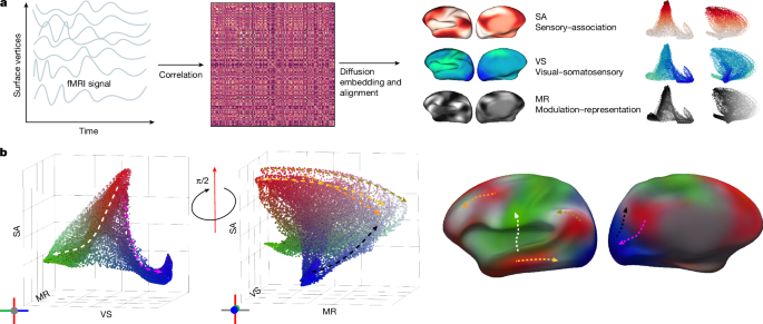
Figure 1 illustrates our analysis framework and aims to establish visualization conventions to facilitate fast and simple interpretations of our lifespan gradients. First, we associate a colour map with each gradient axis. For the SA, VS and MR axes, these gradient-specific colour maps span from white to red, green to blue and black to grey, respectively. To visualize the topography of all three gradients on the cortical surface simultaneously, we devised a colour-mapping scheme that combines the gradient-specific colour maps such that vertices at the association pole of the SA axis are red, vertices at the modulation pole of the MR axis are grey and the visual and somatosensory poles of the VS axis are blue and green, respectively. In Fig. 1b, we display three-dimensional embeddings of all three gradients with our three-dimensional colour map, and establish notation to indicate embedding axis orientation.

Figure 2a uses the aforementioned gradient-specific colour maps to chart topographical progression of each gradient in combination with density plots for gradient value. Note that we use a constant range with respect to time for the colour maps of surface-based gradient plots. Density plots are computed using kernel density estimation (KDE) applied to the vertex-wise GAMM prediction of gradient value at selected time points. Before density estimation, we normalize gradient values across vertices and all time points to range between 0 and 1. To showcase temporal changes in both the shape and the scale of density distribution, we use constant horizontal and vertical axis ranges across time.

In Extended Data Fig. 4 (bottom), we display mean between-network embedding distance in matrix form, in which the mean distance between each network pair is encoded by the colour of that cell.

Reporting summary

Further information on research design is available in the Nature Portfolio Reporting Summary linked to this article.